编程作业2 logistic_regression(逻辑回归)(吴恩达)
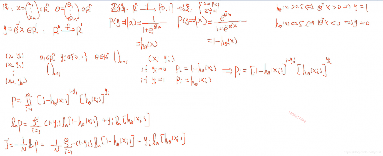
推荐运行环境:python 3.6 建立一个逻辑回归模型来预测一个学生是否被大学录取。根据两次考试的结果来决定每个申请人的录取机会。有以前的申请人的历史数据, 可以用它作为逻辑回归的训练集 python实现逻辑回归 目标:建立分类器(求解出三个参数 θ0 θ1 θ2)即得出分界线 备注:θ1对应’Exam 1’成绩,θ2对应’Exam 2’ 设定阈值,根据阈值判断录取结果 备注:阈值指的是最终得到的概率值.将概率值转化成一个类别.一般是>0.5是被录取了,<0.5未被录取. 实现内容:
sigmoid : 映射到概率的函数 model : 返回预测结果值 cost : 根据参数计算损失 gradient : 计算每个参数的梯度方向 descent : 进行参数更新 accuracy: 计算精度
import pandas as pd
import numpy as np
import matplotlib.pyplot as plt
import seaborn as sns
plt.style.use('fivethirtyeight') #样式美化
import matplotlib.pyplot as plt
from sklearn.metrics import classification_report#这个包是评价报告
1.准备数据
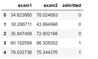
data = pd.read_csv('ex2data1.txt',names = ['exam1', 'exam2', 'admitted'])
data.head() #看前五行
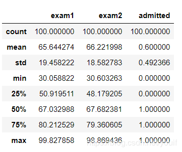
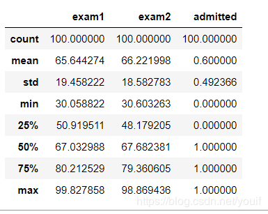
data.describe()
##Error case1 TypeError:unhashable type :_ColorPalette 运行问题更换方案sns.set(context=“notebook”, style=“darkgrid”, palette=sns.color_palette(“RdBu”, 2),color_codes=False) 因为自定义了画板颜色
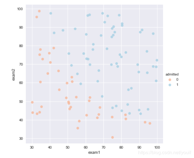
sns.set(context = "notebook",style = "darkgrid",palette = sns.color_palette("RdBu",2)) #设置样式参数,默认主题 darkgrid(灰色背景+白网格),调色板 2色
sns.lmplot('exam1','exam2',hue = 'admitted',data = data, #hue参数是将name所指定的不同类型的数据叠加在一张图中显示
          size = 6,
          fit_reg =False,   #fit_reg'参数,控制是否显示拟合的直线
          scatter_kws = {"s":50})
plt.show()
def get_X(df):#读取特征
#     """
#     use concat to add intersect feature to avoid side effect
#     not efficient for big dataset though
#     """
    ones = pd.DataFrame({'ones': np.ones(len(df))})#ones是m行1列的dataframe
    data = pd.concat([ones, df], axis=1)  # 合并数据,根据列合并 axis = 1的时候,concat就是行对齐,然后将不同列名称的两张表合并 加列
    return data.iloc[:, :-1].values  # 这个操作返回 ndarray,不是矩阵
def get_y(df):#读取标签
#     '''assume the last column is the target'''
    return np.array(df.iloc[:, -1])#df.iloc[:, -1]是指df的最后一列
def normalize_feature(df):
#     """Applies function along input axis(default 0) of DataFrame."""
    return df.apply(lambda column: (column - column.mean()) / column.std())#特征缩放在逻辑回归同样适用
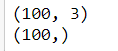
X = get_X(data)
print(X.shape)
y = get_y(data)
print(y.shape)
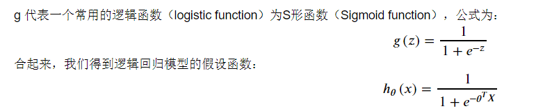
def sigmoid(z):
    return 1 / (1 + np.exp(-z))# your code here  (appro ~ 1 lines)
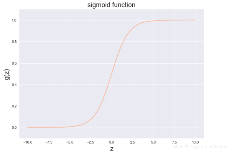
下面程序会调用上面你写好的函数,并画出sigmoid函数图像。如果你的程序正确,你应该能在下方看到函数图像。
fig,ax = plt.subplots(figsize = (8,6))
ax.plot(np.arange(-10,10,step = 0.01),
          sigmoid(np.arange(-10,10,step = 0.01)))
ax.set_ylim((-0.1,1.1))  #lim 轴线显示长度
ax.set_xlabel('z',fontsize=18)
ax.set_ylabel('g(z)',fontsize=18)
ax.set_title('sigmoid function', fontsize=18)
plt.show()

theta = np.zeros(3) # X(m*n) so theta is n*1
theta

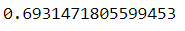
def cost(theta,X,y):
    ''' cost fn is -l(theta) for you to minimize'''
    # your code here  (appro ~ 2 lines)
    return np.mean(-y * np.log(sigmoid(X @ theta)) - (1 - y) * np.log(1 - sigmoid(X @ theta)))
# Hint:X @ theta与X.dot(theta)等价
cost(theta, X, y)
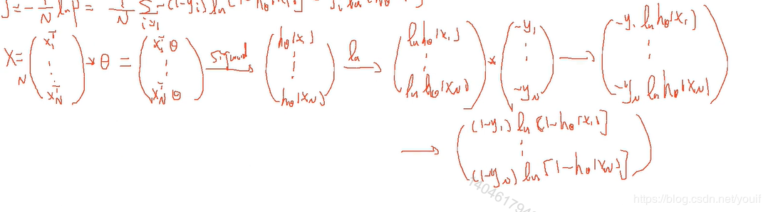
∂J(θ)∂θj=1m∑i=1m(hθ(x(i))−y(i))xj(i)\frac{\partial J\left( \theta \right)}{\partial {{\theta }_{j}}}=\frac{1}{m}\sum\limits_{i=1}^{m}{({{h}_{\theta }}\left( {{x}^{(i)}} \right)-{{y}^{(i)}})x_{_{j}}^{(i)}}∂θj∂J(θ)=m1i=1∑m(hθ(x(i))−y(i))xj(i)
def gradient(theta,X,y):
    # your code here  (appro ~ 2 lines)
    return (1/len(X)) *X.T@(sigmoid(X@theta)-y)
#  return (1 / len(X)) * X.T @ (sigmoid(X @ theta) - y)
gradient(theta, X, y)
![]()
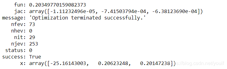
scipy.optimize.minimize 去寻找参数
import scipy.optimize as opt
res =opt.minimize(fun = cost,x0 = theta,args = (X,y), method='Newton-CG', jac=gradient)
##Error case4 The truth value of an array with more than one element is ambiguous. Use a.any() or a.all() Numpy对逻辑表达式判别不清楚, any表示只要有一个True 就返回 True,all表示所有元素为True才会返回True, 否则返回False.
print(res)
def predict(x, theta):
    # your code here  (appro ~ 2 lines)
    prob = sigmoid(x @ theta)
    return (prob >= 0.5).astype(int)   #实现变量类型转换
final_theta = res.x
y_pred = predict(X,final_theta)
print(classification_report(y,y_pred))
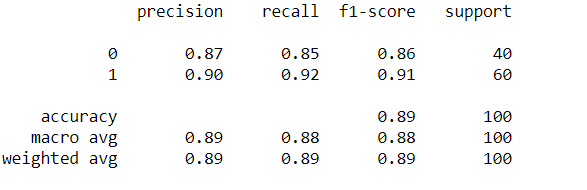
这里涉及评价指标 机器学习中的评价指标(分类指标评Accuracy、Precision、Recall、F1-score、ROC、AUC )(回归指标评价MSE、RMSE、MAE、MAPE、R Squared) 详见这篇文章
7.寻找决策边界http://stats.stackexchange.com/questions/93569/why-is-logistic-regression-a-linear-classifier
X×θ=0X \times \theta = 0X×θ=0 (this is the line)
print(res.x)
![]()
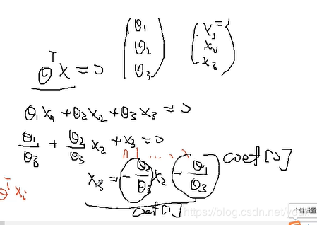
coef = -(res.x / res.x[2])  # find the equation
print(coef)
x = np.arange(130, step=0.1)
y = coef[0] + coef[1]*x
![]()
data.describe()
sns.set(context="notebook", style="ticks", font_scale=1.5) # 默认使用notebook上下文 主题 context可以设置输出图片的大小尺寸(scale)
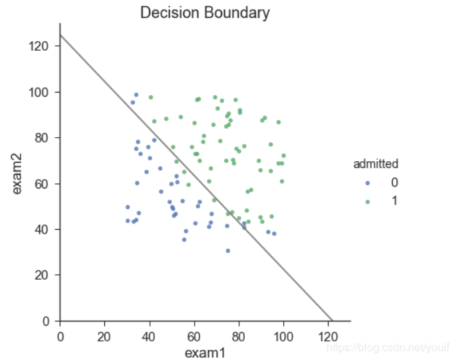
sns.lmplot('exam1', 'exam2', hue='admitted', data=data,
size=6,
fit_reg=False,
scatter_kws={"s": 25}
)
plt.plot(x, y, 'grey')
plt.xlim(0, 130)
plt.ylim(0, 130)
plt.title('Decision Boundary')
plt.show()


数据源码:https://github.com/XiangLinPro/MLPractice
所有巧合的是要么是上天注定要么是一个人偷偷的在努力。

个人微信公众号,专注于学习资源、笔记分享,欢迎关注。我们一起成长,一起学习。一直纯真着,善良着,温情地热爱生活,,如果觉得有点用的话,请不要吝啬你手中点赞的权力,谢谢我亲爱的读者朋友。

The journey of life is like this: idling away a lot of time in befuddlement and growing up in a few moments.
人生的旅程就是这样,用大把时间迷茫 ,在几个瞬间成长。
2020年4月17日于重庆城口
好好学习,天天向上,终有所获
作者:五角钱的程序员