jupyter使用Python编程----使用梯度下降法求多元函数的极值和系数并与最小二乘法进行比较
偏导数:就是对函数的两个未知数求微分
然后得到的函数
例如一个函数为y=x12+x22+2x1x2
d(y)/d(x1)=2x1+2x2
d(y)/d(x2)=2x2+2x1
学习率:
也称为迭代的步长,优化函数的梯度是不断变化的,有时候变化很大,有时候变化很小,所以需要将每次的梯度变化控制在一个合适的范围内。
梯度:
梯度其实就是函数的变化率,在多元函数中,梯度变为了向量,有了变化的方向。
梯度的方向表示的是函数增加最快的方向。
梯度下降法求解,首先就要求得所给定函数的偏导数,即y对x1和x2的微分函数,规定学习率,给定一组初始值,然后计算梯度函数,使用迭代公式更新迭代一次后的函数未知数的值,然后计算出迭代后的梯度函数,将原梯度函数的值与迭代后的梯度函数的值的差值进行判断,判断差值是否收敛,若收敛,就停止算法,否则,就重复之前的迭代。
1、首先导入需要的库并设置字符集
import numpy as np
import matplotlib as mpl
import matplotlib.pyplot as plt
from mpl_toolkits.mplot3d import Axes3D
# 设置字符集,防止中文乱码
mpl.rcParams['font.sans-serif'] = [u'simHei']
mpl.rcParams['axes.unicode_minus'] = False
2、对函数用MATLAB进行显示
#定义要求极值的函数表达式
def f2(x1,x2):
return x1**2+2*x2**2-4*x1-2*x1*x2
X1 = np.arange(0,5,0.1)
X2 = np.arange(0,5,0.1)
X1, X2 = np.meshgrid(X1, X2) # 生成xv、yv,将X1、X2变成n*m的矩阵,方便后面绘图
Y = np.array(list(map(lambda t : f2(t[0],t[1]),zip(X1.flatten(),X2.flatten()))))
Y.shape = X1.shape
%matplotlib inline
#作图
fig = plt.figure(facecolor='w')
ax = Axes3D(fig)
ax.plot_surface(X1,X2,Y,rstride=1,cstride=1,cmap=plt.cm.jet)
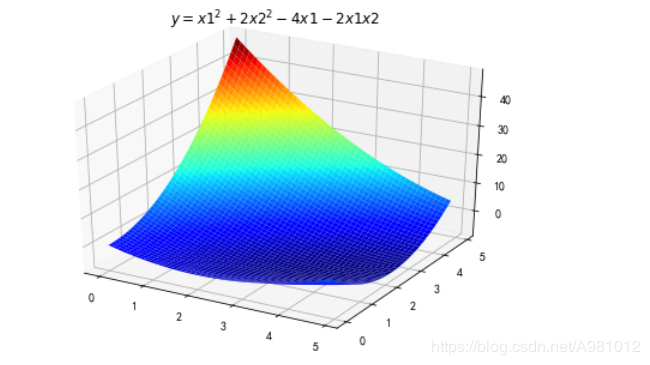
ax.set_title(u'$ y = x1^2 +2x2^2-4x1-2x1x2 $')
plt.show()
显示为:
3、用梯度下降法求解函数极值,要求对应x1和x2的偏导数
#函数
def f2(x, y):
    return x**2+2*y**2-4*x-2*x*y
## 求两个未知数对于函数的偏导数
def hx1(x, y):
    return 2*x-2*y-4
def hx2(x, y):
    return -2*x+4*y
4、定义初值和学习率,然后运用数组保存梯度下降后所经过的点
#学习率
alpha = 0.1
#保存梯度下降经过的点
GD_X1 = []
GD_X2 = []
GD_Y = []
GD_X1.append(x1)
GD_X2.append(x2)
GD_Y.append(f2(x1,x2))
# 定义y的变化量和迭代次数
y_change = 0-f2(x1,x2)
iter_num = 0
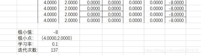
5、判断前后两次迭代的y值的差值,如果很小表明函数已经收敛了,就可以得出最后的极小值了,然后用MATLAB显示出所经过的点,我的图上经过的点在背面有点儿看不清晰
while(y_change > 1e-10) :
tmp_x1 = x1 - alpha * hx1(x1,x2)
tmp_x2 = x2 - alpha * hx2(x1,x2)
tmp_y = f2(tmp_x1,tmp_x2)
y_change =f2(x1,x2)-tmp_y
x1 = tmp_x1
x2 = tmp_x2
GD_X1.append(x1)
GD_X2.append(x2)
GD_Y.append(tmp_y)
iter_num =iter_num+1
print(u"最终结果为:(%.5f, %.5f, %.5f)" % (x1, x2, f2(x1,x2)))
print(u"迭代过程中X的取值,迭代次数:%d" % iter_num)
print(GD_X1)#打印出迭代的x1的值
# 作图
fig = plt.figure(facecolor='w',figsize=(20,18))
ax = Axes3D(fig)
ax.plot_surface(X1,X2,Y,rstride=1,cstride=1,cmap=plt.cm.jet)
ax.plot(GD_X1,GD_X2,GD_Y,'ko-')
ax.set_xlabel('x')
ax.set_ylabel('y')
ax.set_zlabel('z')
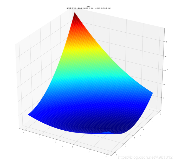
ax.set_title(u'函数;\n学习率:%.3f; 最终解:(%.3f, %.3f, %.3f);迭代次数:%d' % (alpha, x1, x2, f2(x1,x2), iter_num))
plt.show()
得到的结果以及显示为:
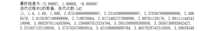
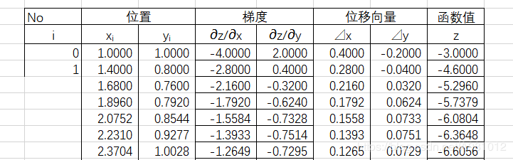
6、根据结果显示可以看出,用Python实现的梯度下降求多元函数的极值精度是要比excel求得的要小一点的
完整代码为:
import numpy as np
import matplotlib as mpl
import matplotlib.pyplot as plt
from mpl_toolkits.mplot3d import Axes3D
# 设置字符集,防止中文乱码
mpl.rcParams['font.sans-serif'] = [u'simHei']
mpl.rcParams['axes.unicode_minus'] = False
def f2(x1,x2):
    return x1**2+2*x2**2-4*x1-2*x1*x2
X1 = np.arange(0,5,0.1)
X2 = np.arange(0,5,0.1)
X1, X2 = np.meshgrid(X1, X2) # 生成xv、yv,将X1、X2变成n*m的矩阵,方便后面绘图
Y = np.array(list(map(lambda t : f2(t[0],t[1]),zip(X1.flatten(),X2.flatten()))))
Y.shape = X1.shape # 1600的Y图还原成原来的(40,40)
%matplotlib inline
#作图
fig = plt.figure(facecolor='w')
ax = Axes3D(fig)
ax.plot_surface(X1,X2,Y,rstride=1,cstride=1,cmap=plt.cm.jet)
ax.set_title(u'$ y = x1^2 +2x2^2-4x1-2x1x2 $')
plt.show()
#函数
def f2(x, y):
    return x**2+2*y**2-4*x-2*x*y
## 求两个未知数对于函数的偏导数
def hx1(x, y):
    return 2*x-2*y-4
def hx2(x, y):
    return -2*x+4*y
x1 = 1
x2 = 1
#学习率
alpha = 0.1
#保存梯度下降经过的点
GD_X1 = []
GD_X2 = []
GD_Y = []
GD_X1.append(x1)
GD_X2.append(x2)
GD_Y.append(f2(x1,x2))
# 定义y的变化量和迭代次数
y_change = 0-f2(x1,x2)
iter_num = 0
while(y_change > 1e-10) :
    tmp_x1 = x1 - alpha * hx1(x1,x2)
    tmp_x2 = x2 - alpha * hx2(x1,x2)
    tmp_y = f2(tmp_x1,tmp_x2)
    y_change =f2(x1,x2)-tmp_y
    x1 = tmp_x1
    x2 = tmp_x2
    GD_X1.append(x1)
    GD_X2.append(x2)
    GD_Y.append(tmp_y)
    iter_num =iter_num+1
print(u"最终结果为:(%.5f, %.5f, %.5f)" % (x1, x2, f2(x1,x2)))
print(u"迭代过程中X的取值,迭代次数:%d" % iter_num)
print(GD_X1)
# 作图
fig = plt.figure(facecolor='w',figsize=(20,18))
ax = Axes3D(fig)
ax.plot_surface(X1,X2,Y,rstride=1,cstride=1,cmap=plt.cm.jet)
ax.plot(GD_X1,GD_X2,GD_Y,'ko-')
ax.set_xlabel('x')
ax.set_ylabel('y')
ax.set_zlabel('z')
ax.set_title(u'函数;\n学习率:%.3f; 最终解:(%.3f, %.3f, %.3f);迭代次数:%d' % (alpha, x1, x2, f2(x1,x2), iter_num))
plt.show()
梯度下降法求解多元函数的系数
1、导入需要的库并读取数据
import numpy as np
from matplotlib import pyplot as plt
from mpl_toolkits.mplot3d import Axes3D
data=np.genfromtxt('./yingyee.csv',delimiter=',')
x_data=data[:,:-1]
y_data=data[:,2]
2、定义学习率和各个系数初值以及最大迭代次数
#定义学习率、斜率、截据
#设方程为y=theta1*x1+theta2*x2+theta0
lr=0.00001
theta0=0
theta1=0
theta2=0
#定义最大迭代次数,因为梯度下降法是在不断迭代更新k与b
epochs=10000
3、定义损失函数
#定义最小二乘法函数-损失函数(代价函数)
def compute_error(theta0,theta1,theta2,x_data,y_data):
    totalerror=0
    for i in range(0,len(x_data)):#定义一共有多少样本点
        totalerror=totalerror+(y_data[i]-(theta1*x_data[i,0]+theta2*x_data[i,1]+theta0))**2
    return totalerror/float(len(x_data))/2
4、定义函数进行梯度下降算法求解参数
#梯度下降算法求解参数
def gradient_descent_runner(x_data,y_data,theta0,theta1,theta2,lr,epochs):
    m=len(x_data)
    for i in range(epochs):
        theta0_grad=0
        theta1_grad=0
        theta2_grad=0
        for j in range(0,m):
            theta0_grad-=(1/m)*(-(theta1*x_data[j,0]+theta2*x_data[j,1]+theta2)+y_data[j])
            theta1_grad-=(1/m)*x_data[j,0]*(-(theta1*x_data[j,0]+theta2*x_data[j,1]+theta0)+y_data[j])
            theta2_grad-=(1/m)*x_data[j,1]*(-(theta1*x_data[j,0]+theta2*x_data[j,1]+theta0)+y_data[j])
        theta0=theta0-lr*theta0_grad
        theta1=theta1-lr*theta1_grad
        theta2=theta2-lr*theta2_grad
    return theta0,theta1,theta2
5、求解表示出方程
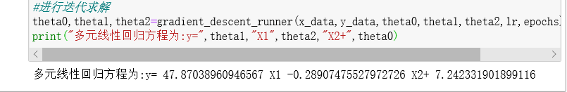
#进行迭代求解
theta0,theta1,theta2=gradient_descent_runner(x_data,y_data,theta0,theta1,theta2,lr,epochs)
print("多元线性回归方程为:y=",theta1,"X1",theta2,"X2+",theta0)
得到的结果为:
完整代码为:
import numpy as np
from matplotlib import pyplot as plt
from mpl_toolkits.mplot3d import Axes3D
data=np.genfromtxt('./yingyee.csv',delimiter=',')
x_data=data[:,:-1]
y_data=data[:,2]
#定义学习率、斜率、截据
#设方程为y=theta1*x1+theta2*x2+theta0
lr=0.00001
theta0=0
theta1=0
theta2=0
#定义最大迭代次数,因为梯度下降法是在不断迭代更新k与b
epochs=10000
#定义最小二乘法函数-损失函数(代价函数)
def compute_error(theta0,theta1,theta2,x_data,y_data):
    totalerror=0
    for i in range(0,len(x_data)):#定义一共有多少样本点
        totalerror=totalerror+(y_data[i]-(theta1*x_data[i,0]+theta2*x_data[i,1]+theta0))**2
    return totalerror/float(len(x_data))/2
    #梯度下降算法求解参数
def gradient_descent_runner(x_data,y_data,theta0,theta1,theta2,lr,epochs):
    m=len(x_data)
    for i in range(epochs):
        theta0_grad=0
        theta1_grad=0
        theta2_grad=0
        for j in range(0,m):
            theta0_grad-=(1/m)*(-(theta1*x_data[j,0]+theta2*x_data[j,1]+theta2)+y_data[j])
            theta1_grad-=(1/m)*x_data[j,0]*(-(theta1*x_data[j,0]+theta2*x_data[j,1]+theta0)+y_data[j])
            theta2_grad-=(1/m)*x_data[j,1]*(-(theta1*x_data[j,0]+theta2*x_data[j,1]+theta0)+y_data[j])
        theta0=theta0-lr*theta0_grad
        theta1=theta1-lr*theta1_grad
        theta2=theta2-lr*theta2_grad
    return theta0,theta1,theta2
#进行迭代求解
theta0,theta1,theta2=gradient_descent_runner(x_data,y_data,theta0,theta1,theta2,lr,epochs)
print("多元线性回归方程为:y=",theta1,"X1",theta2,"X2+",theta0)
最小二乘法求解多元函数的系数
基本原理参考:https://blog.csdn.net/A981012/article/details/105105318.
1、导入需要的库
import pandas as pd
import numpy as np
import math
import matplotlib.pyplot as plt
2、准备数据
#准备数据
p=pd.read_excel('yingyee.xlsx')
x1=p["店铺的面积"]
x2=p["距离最近的车站"]
x=p[["店铺的面积","距离最近的车站"]]
y=p["月营业额"]
3、使用矩阵进行运算求出各个系数的解
n=10#数据个数
h=[]
for i in range(n):
    values=[]
    values.append(1)
    values.append(x1[i])
    values.append(x2[i])
    h.append(values)
h0=np.array(h)#将h0数组化
h1=np.array(h0).T#h1为h的转置矩阵
h2=h1@h0
h3=np.linalg.inv(h2)#求逆矩阵
temp=h3@h1@y
#temp=np.mat(temp)
temp
w0=temp[0]
w1=temp[1]
w2=temp[2]
print("线性回归方程为:y=",w1,"x1",w2,"x2+",w0)
所得到的结果为:
完整代码为:
import pandas as pd
import numpy as np
from sklearn import linear_model
import matplotlib.pyplot as plt
import sklearn.metrics as sm
#准备数据
p=pd.read_excel('yingyee.xlsx')
x=p[["店铺的面积","距离最近的车站"]]
x1=p["店铺的面积"]
x2=p["距离最近的车站"]
y=p["月营业额"]
n=10#数据个数
h=[]
for i in range(n):
    values=[]
    values.append(1)
    values.append(x1[i])
    values.append(x2[i])
    h.append(values)
h0=np.array(h)#将h0数组化
h1=np.array(h0).T#h1为h的转置矩阵
h2=h1@h0
h3=np.linalg.inv(h2)#求逆矩阵
temp=h3@h1@y
#temp=np.mat(temp)
temp
w0=temp[0]
w1=temp[1]
w2=temp[2]
print("线性回归方程为:y=",w1,"x1",w2,"x2+",w0)
比较和总结
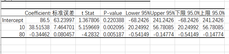
用excel对数据进行多元回归,可得出
梯度下降法求解得出的系数为:
最小二乘法求解得出的系数为:
这两种方法得到的结果与excel得到的结果对比,最小二乘法所得的结果更贴近于excel,所以最小二乘法的结果要准确一些。梯度下降法求解极值要好一些,而求解多元函数的系数还是用最小二乘法要好一些。
参考博客:
https://www.jianshu.com/p/17116b9e4322.
https://blog.csdn.net/qq_35946969/article/details/84446000.
https://www.cnblogs.com/LOSKI/p/10639733.html
https://www.jianshu.com/p/424b7b70df7b…
作者:混混度日的咸鱼