Python 普通最小二乘法(OLS)进行多项式拟合的方法

Ruth ·

更新时间:2024-09-21

· 524 次阅读

多元函数拟合。如电视机和收音机价格多销售额的影响，此时自变量有两个。

python 解法：


import numpy as np
import pandas as pd
#import statsmodels.api as sm #方法一
import statsmodels.formula.api as smf #方法二
import matplotlib.pyplot as plt
from mpl_toolkits.mplot3d import Axes3D
df = pd.read_csv('http://www-bcf.usc.edu/~gareth/ISL/Advertising.csv', index_col=0)
X = df[['TV', 'radio']]
y = df['sales']
#est = sm.OLS(y, sm.add_constant(X)).fit() #方法一
est = smf.ols(formula='sales ~ TV + radio', data=df).fit() #方法二
y_pred = est.predict(X)
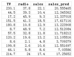
df['sales_pred'] = y_pred
print(df)
print(est.summary()) #回归结果
print(est.params) #系数
fig = plt.figure()
ax = fig.add_subplot(111, projection='3d') #ax = Axes3D(fig)
ax.scatter(X['TV'], X['radio'], y, c='b', marker='o')
ax.scatter(X['TV'], X['radio'], y_pred, c='r', marker='+')
ax.set_xlabel('X Label')
ax.set_ylabel('Y Label')
ax.set_zlabel('Z Label')
plt.show()

Python 普通最小二乘法(OLS)进行多项式拟合

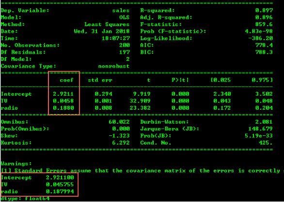
拟合的各项评估结果和参数都打印出来了，其中结果函数为：

f(sales) = β0 + β1*[TV] + β2*[radio]

f(sales) = 2.9211 + 0.0458 * [TV] + 0.188 * [radio]

Python 普通最小二乘法(OLS)进行多项式拟合

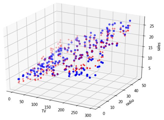
图中，sales 方向上，蓝色点为原 sales 实际值，红色点为拟合函数计算出来的值。其实误差并不大，部分数据如下。

Python 普通最小二乘法(OLS)进行多项式拟合

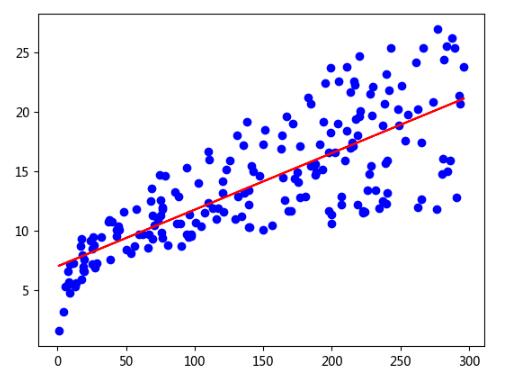
同样可拟合一元函数;


import numpy as np
import pandas as pd
import statsmodels.formula.api as smf
import matplotlib.pyplot as plt
from mpl_toolkits.mplot3d import Axes3D
df = pd.read_csv('http://www-bcf.usc.edu/~gareth/ISL/Advertising.csv', index_col=0)
X = df['TV']
y = df['sales']
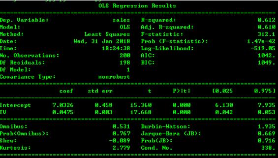
est = smf.ols(formula='sales ~ TV ', data=df).fit()
y_pred = est.predict(X)
print(est.summary())
fig = plt.figure()
ax = fig.add_subplot(111)
ax.scatter(X, y, c='b')
ax.plot(X, y_pred, c='r')
plt.show()

Python 普通最小二乘法(OLS)进行多项式拟合

Ridge Regression:（岭回归交叉验证）

岭回归(ridge regression, Tikhonov regularization)是一种专用于共线性数据分析的有偏估计回归方法，实质上是一种改良的最小二乘估计法，通过放弃最小二乘法的无偏性，以损失部分信息、降低精度为代价获得回归系数更为符合实际、更可靠的回归方法，对病态数据的拟合要强于最小二乘法。通常岭回归方程的R平方值会稍低于普通回归分析，但回归系数的显著性往往明显高于普通回归，在存在共线性问题和病态数据偏多的研究中有较大的实用价值。


import numpy as np
import pandas as pd
import matplotlib.pyplot as plt
from sklearn import linear_model
from mpl_toolkits.mplot3d import Axes3D
df = pd.read_csv('http://www-bcf.usc.edu/~gareth/ISL/Advertising.csv', index_col=0)
X = np.asarray(df[['TV', 'radio']])
y = np.asarray(df['sales'])
clf = linear_model.RidgeCV(alphas=[i+1 for i in np.arange(200.0)]).fit(X, y)
y_pred = clf.predict(X)
df['sales_pred'] = y_pred
print(df)
print("alpha=%s, 常数=%.2f, 系数=%s" % (clf.alpha_ ,clf.intercept_,clf.coef_))
fig = plt.figure()
ax = fig.add_subplot(111, projection='3d')
ax.scatter(df['TV'], df['radio'], y, c='b', marker='o')
ax.scatter(df['TV'], df['radio'], y_pred, c='r', marker='+')
ax.set_xlabel('TV')
ax.set_ylabel('radio')
ax.set_zlabel('sales')
plt.show()

输出结果：alpha=150.0, 常数=2.94, 系数=[ 0.04575621 0.18735312]

以上这篇Python 普通最小二乘法(OLS)进行多项式拟合的方法就是小编分享给大家的全部内容了，希望能给大家一个参考，也希望大家多多支持软件开发网。

您可能感兴趣的文章:Python实现的多项式拟合功能示例【基于matplotlib】Python 确定多项式拟合/回归的阶数实例Python多项式回归的实现方法详解Pytorch 使用Pytorch拟合多项式(多项式回归)在python中利用numpy求解多项式以及多项式拟合的方法

最小二乘法方法多项式拟合 Python

1024 个赞