机器学习代码实战——PCA（主成分分析）

Efia ·

更新时间:2024-09-21

· 685 次阅读

文章目录1.主成分分析基本概念2.代码 1.主成分分析基本概念

在这里插入图片描述

2.代码

导入必要的库

import pandas as pd
import numpy as np
from sklearn.datasets import load_iris  #sklearn中导入load_iris数据
import matplotlib.pyplot as plt
from sklearn.preprocessing import StandardScaler
%matplotlib inline

加载数据，构建DataFrame

iris = load_iris()    #加载数据集
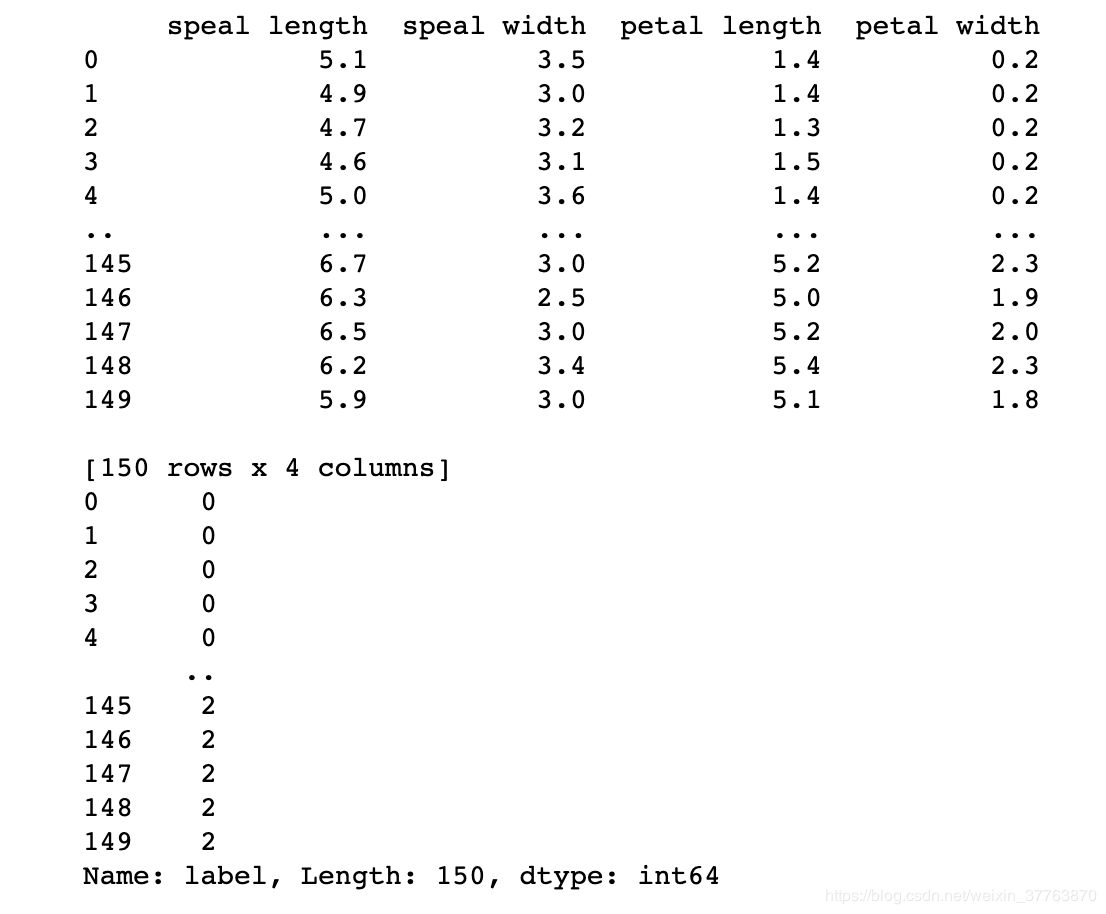
df = pd.DataFrame(iris.data, columns = iris.feature_names)   #创建DataFrame对象
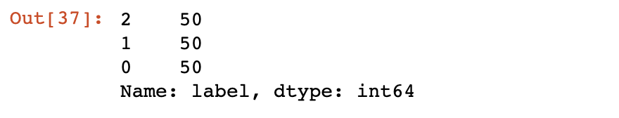
df['label'] = iris.target	 #iris.target是标签
df.columns = ['speal length','speal width', 'petal length', 'petal width', 'label']
df.label.value_counts()	#统计不同标签的个数

在这里插入图片描述

X = df.iloc[:,0:4]        #对df进行切分第0、1、2、3列为X
print(X)
y = df.iloc[:,4]          #第4列为Y
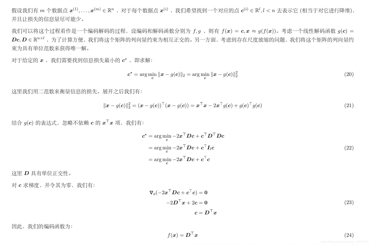
print(y)

在这里插入图片描述
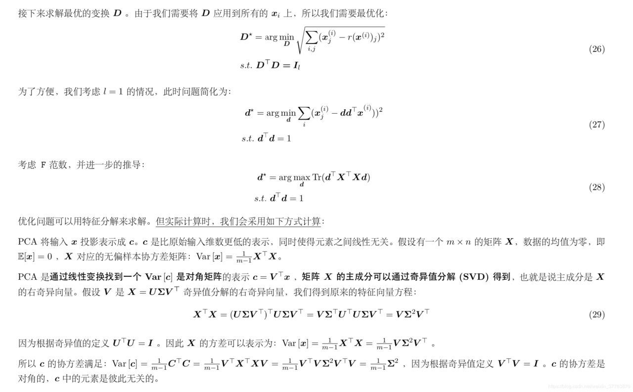
在scikit-learn中，与PCA相关的类都在sklearn.decomposition包中。最常用的PCA类就是sklearn.decomposition.PCA
PCA类基本不需要调参，一般来说，我们只需要指定我们需要降维到的维度，或者我们希望降维后的主成分的方差和占原始维度所有特征方差和的比例阈值就可以了

sklearn_pca = sklearnPCA(n_components = 2)       #n_components这个参数可以帮我们指定希望PCA降维后的特征维度数目(PCA算法中所要保留的主成分个数n，也即保留下来的特征个数n)
Y = sklearn_pca.fit_transform(X)         #用X来训练PCA模型，同时返回降维后的数据

构建主成分分析后的数据

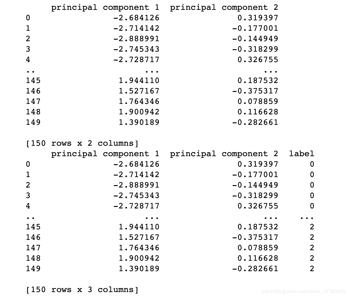
principalDf = pd.DataFrame(data = np.array(Y),columns = ['principal component 1','principal component 2'])   
print(principalDf)
Df = pd.concat([principalDf,y],axis = 1) #需要连接的对象，eg [df1, df2]  #axis = 0, 表示在水平方向(row)进行连接 axis = 1, 表示在垂直方向(column)进行连接 
print(Df)

在这里插入图片描述
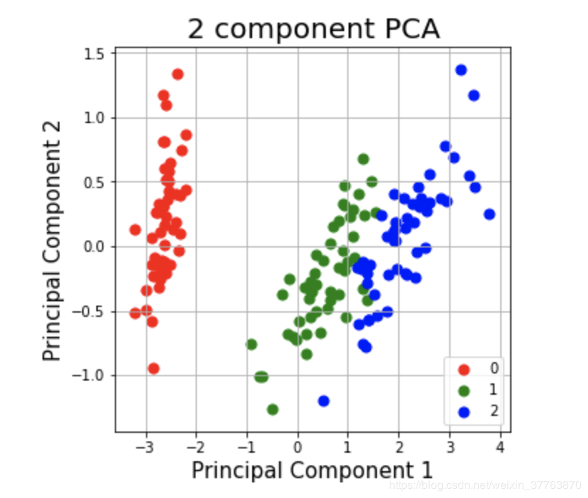
画出主成分分析后的散点图

fig = plt.figure(figsize = (5,5))     #控制图片大小
ax = fig.add_subplot(1,1,1)      #“111”表示“1×1网格，第一子图”，“234”表示“2×3网格，第四子图”。
ax.set_xlabel('Principal Component 1',fontsize = 15)
ax.set_ylabel('Principal Component 2',fontsize = 15)
ax.set_title('2 component PCA',fontsize = 20)
targets = [0,1,2]
colors = ['r', 'g', 'b']
for target, color in zip(targets, colors):   #zip() 函数用于将可迭代的对象作为参数，将对象中对应的元素打包成一个个元组，然后返回由这些元组组成的列表。
    indicesToKeep = Df['label'] == target
    ax.scatter(Df.loc[indicesToKeep,'principal component 1'],Df.loc[indicesToKeep,'principal component 2'], c = color ,s = 50)
ax.legend(targets)
ax.grid()

在这里插入图片描述