机器学习-支持向量机(Support Vector Machine)
Another powerful and widely used learning algorithm is the Support Vector Machine (SVM), which can be considered an extension of the perceptron. Using the perceptron algortihm, misclassification errors is our target to be optimized. However, for SVM, our optimization objective is to maximize the margin. The margin is defined as the distance between the separating hyperplance (decision boundary) and the training samples that are closest to this hyperplance, which are the so-called support vectors.
From
Sebastian Raschka, Vahid Mirjalili. Python机器学习第二版. 南京:东南大学出版社,2018.
import matplotlib.pyplot as plt
from sklearn import datasets
import numpy as np
from sklearn.model_selection import train_test_split
from sklearn.preprocessing import StandardScaler
from sklearn.svm import SVC
from SupportVectorMachine.visualize_test_idx import plot_decision_regions
plt.rcParams['figure.dpi']=200
plt.rcParams['savefig.dpi']=200
font = {'family': 'Times New Roman',
'weight': 'light'}
plt.rc("font", **font)
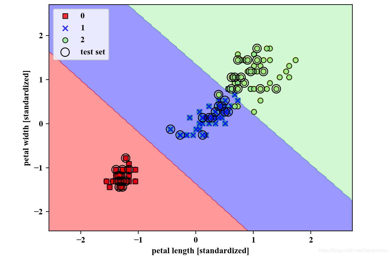
##Section 1: Load data and split it into train/test dataset
iris=datasets.load_iris()
X=iris.data[:,[2,3]]
y=iris.target
X_train,X_test,y_train,y_test=train_test_split(X,y,test_size=0.3,random_state=1,stratify=y)
#Section 2: Preprocessing data in standardized
sc=StandardScaler()
sc.fit(X_train)
X_train_std=sc.transform(X_train)
X_test_std=sc.transform(X_test)
X_combined_std=np.vstack((X_train_std,X_test_std))
y_combined=np.hstack((y_train,y_test))
#Section 3: Train SVC classifier via Sklearn
svm=SVC(kernel='linear',C=1.0,random_state=1)
svm.fit(X_train_std,y_train)
plot_decision_regions(X=X_combined_std,
y=y_combined,
classifier=svm,
test_idx=range(105,150))
plt.xlabel('petal length [standardized]')
plt.ylabel('petal width [standardized]')
plt.legend(loc='upper left')
plt.savefig('./fig1.png')
plt.show()
备注:
plot_decision_regions如果不作特别说明,均为机器学习-感知机(Perceptron)-Scikit-Learn中的plot_decision_regions函数,链接为:机器学习-感知机(Perceptron)-Scikit-Learn。
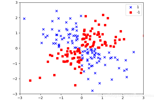
第一部分:构造非线性的与非问题数据集
#Section 1: Construct nonlinear "logic_or" dataset
import matplotlib.pyplot as plt
import numpy as np
np.random.seed(1)
X_xor=np.random.randn(200,2)
y_xor=np.logical_xor(X_xor[:,0]>0,
                     X_xor[:,1]>0)
y_xor=np.where(y_xor,1,-1)
plt.scatter(X_xor[y_xor==1,0],
            X_xor[y_xor==1,1],
            c='b',
            marker='x',
            label='1')
plt.scatter(X_xor[y_xor==-1,0],
            X_xor[y_xor==-1,1],
            c='r',
            marker='s',
            label='-1')
plt.xlim([-3,3])
plt.ylim([-3,3])
plt.legend(loc='best')
plt.savefig('./fig2.png')
plt.show()
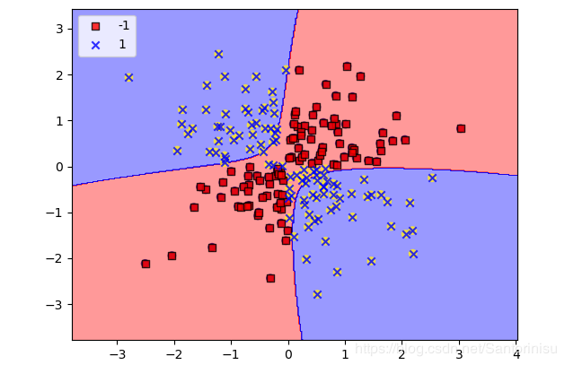
第二部分:Cut-Off参数对划分边界的影响
#Section 2: Train SVC Classifier on Non-linear Model
#Section 2.1: Smaller gamma: "cut-off parameter for Gaussian sphere"
#             Used to soften or tighten the decision boundary
from SupportVectorMachine.visualize import plot_decision_regions
svm=SVC(kernel='rbf',random_state=1,gamma=0.10,C=10.0)
svm.fit(X_xor,y_xor)
plot_decision_regions(X_xor,y_xor,classifier=svm)
plt.legend(loc='upper left')
plt.savefig('./fig3.png')
plt.show()
#Section 2.2: Larger gamma
svm=SVC(kernel='rbf',random_state=1,gamma=100,C=10.0)
svm.fit(X_xor,y_xor)
plot_decision_regions(X_xor,y_xor,classifier=svm)
plt.legend(loc='upper left')
plt.savefig('./fig4.png')
plt.show()
Gamma参数:
Gamma=0.1的场景:
Gamma=100的场景:
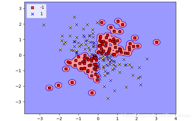
值得注意,Gamma参数为Gauss核函数的自由参数,C为正则化参数。由于核函数的引入,将低维空间不可分的问题转化到线性可分的高维空间。然而,映射到高维空间将使得特征空间的转换和距离计算将不可避免地导致计算量增大。因此,核函数的引入主要在于应用低维空间的特征计算高维空间的距离量。
Roughly Spearking, the term kernel can be interpreted as a similarity function between a pair of samples. The minus sign inverts the distance measure into a similarity score, and, due to the exponential term, the resulting similarity score will fall into a range between 1 (for exactly similar sample) and 0 (for very dissimilar samples).
From
Sebastian Raschka, Vahid Mirjalili. Python机器学习第二版. 南京:东南大学出版社,2018.
参考文献:
Sebastian Raschka, Vahid Mirjalili. Python机器学习第二版. 南京:东南大学出版社,2018.
作者:Santorinisu