卡尔曼滤波器在移动机器人定位中的应用(上)
一个人的喜欢就是把自己对偶然间闪过的念想坚持,直到它变成一种习惯。——xiahouzuoxin
说实话,这样的人生确实比较有趣,但这个句子不是我说的。在下面,凭借着人类特有的懦弱与阿Q精神,任何人都可以被迫做到:)
我可以做到把自己持久性的不喜欢坚持,直到它变成一种习惯和喜欢。——肥鼠路易 Overview and MotivationThe study of mobile robots is an intrinsically interdisciplinary research area involving the following:
Mechanical engineering—vehicle design and in particular locomotive mechanisms.
Computer science—representation,sensing,and planning algorithms.
Electrical engineering—system integration,sensors,and communications.
Cognitive psychology,perception,and neuroscience—insights on how biological organisms solve similar problems.
绝对位移传感器:输出是相对于一个绝对(固定)参考点的位置,传感器断电再恢复供电时,无需复位
相对位移传感器:增量式位移传感器(如增量式编码器,增量式光栅尺),断电后需要进行系统复位,才能继续测量。
位移与加速度是可以互相转换的。加速度传感器测得的数据经二次积分处理,得到的就是位移量,同样的位移传感器测得的数据经二次微分处理,得到的数据为加速度值。其实不管使用加速度测量位移或者位移测量加速度在实际应用中都非常少见,主要原因信号转换过程要求采集系统必须具备相应的微分或者积分运算能力,而不管位移传感器或者加速度传感器都是极为常用的产品,还不如直接选用相关的传感器去测量对应的物理量划算。
--------------------------------------------------------------------------- ——作者:米朗位移传感器
思考移动机器人的定位问题:假设我们的移动机器人只在平面上移动,那么要确定的无非是机器人的位置和转向
X=[x,y,θ]TX=[x,y,\theta]^TX=[x,y,θ]T
在这里,我们运用机器人定位研究领域中最常见的算法,卡尔曼滤波器。
TA的典型实例从一组有限的,包含噪声的,通过对物体位置的观察序列(可能有偏差)预测出物体的位置的坐标及速度。
卡尔曼滤波模型假设(k+1)时刻的真实状态Xk+1X_{k+1}Xk+1是从k时刻的状态XkX_kXk演化而来。(相关矩阵符号含义见维基百科)
Xk+1=Fx+1Xk+Bk+1uk+1+wk+1X_{k+1} = F_{x+1}X_k+B_{k+1}u_{k+1}+w_{k+1}Xk+1=Fx+1Xk+Bk+1uk+1+wk+1
Zk+1=Hk+1Xk+1+vk+1Z_{k+1} = H_{k+1}X_{k+1}+v_{k+1}Zk+1=Hk+1Xk+1+vk+1
其中,Fx+1F_{x+1}Fx+1相当于是状态转移矩阵。FkF_kFk和BkB_kBk是需要我们来确定的。
The equations for the Kalman filter fall into two groups:
time update equations and measurement update equations.
The time update equations are responsible for projecting forward (in time) the current state and error covariance estimates to obtain the a priori estimates for the next time step.
The measurement update equations are responsible for the feedback—i.e. for incorporating a new measurement into the a priori estimate to obtain an improved a posteriori estimate.
(注释:我们还可以把这时间更新方程和测量更新方程分别看作预测前向传递与反馈更正。)
卡尔曼滤波是一种递归的估计,由于TA建立在隐式马尔科夫的基础上,TA只要获知上一时刻状态的估计值以及当前状态的观测值就可以计算出当前状态的估计值,因此不需要记录观测或者估计的历史信息。比较有趣的一点是,TA的名字虽然含有“滤波器”,但TA是完全作用在时域上的。
卡尔曼滤波器的状态由以下两个变量表示:
X^k∣k{\displaystyle {\hat {\textbf {X}}}_{k|k}}X^k∣k:在时刻k的状态的估计;
Pk∣k{\displaystyle {\textbf {P}}_{k|k}}Pk∣k:后验估计误差协方差矩阵,度量估计值的精确程度。
基本卡尔曼滤波器(The basic Kalman filter)是限制在线性的假设之下。然而,大部分非平凡的(non-trivial)的系统都是非线性系统。其中的“非线性性质”(non-linearity)可能是伴随存在过程模型(process model)中或观测模型(observation model)中,或者两者兼有之。
扩展卡尔曼滤波器(Extended Kalman Filter,简称EKF)中状态转换和观测模型不需要是状态的线性函数,可替换为(可微的)函数。 这个过程,实质上将非线性的函数在当前估计值处线性化
啊啊啊,偶然遇到的一个名人名言,摘抄下来:
We are like dwarfs on the shoulders of giants, by whose grace we see farther than they. Our study of the works of the ancients enables us to give fresh life to their finer ideas, and rescue them from time’s oblivion and man’s neglect.
-----------------------------------------------------------------—— Peter of Blois, late twelfth century
如果想要追溯卡尔曼滤波器的历史,我们需要穿越会17世纪追寻那些闪耀巨人们的脚步,至于身份呢,我们全且当一当小矮人,好不好:)
在这次旅行中,我觉察到现阶段我对于卡尔曼滤波器与占星预测学关系的研究竟然还真的有一丢丢的联系哇,因为卡尔曼滤波器最开始的思想雏形来源于天文学家对于天体的运动估计。(PS:科普一下占星与天文的关系,最开始,占星学与天文学是不分家的,后来逐渐分流,区分于天文学,占星学是基于地心说的主观经验世界预测:)
刚开始看的时候,先验估计状态,后验估计状态,先验估计误差,后验估计误差,只想变成猪八戒大叫“师傅,大师兄,这些公式都是什么妖魔鬼怪!!大师兄,救我!!!”
推导卡尔曼公式,我们的目的不过是寻找一个方程式来计算后验估计状态变量x^k\hat x_kx^k,后验估计状态变量x^k\hat x_kx^k是先验估计状态变量x^k−\hat x_k^-x^k−还有真实测量值zkz_kzk与测量预测Hxk−Hx_k^-Hxk−之间偏差的线性结合。
x^k=x^k−+K(zk−Hx^k−)\hat x_k = \hat x_k^{-} + K(z_k - H\hat x_k^-)x^k=x^k−+K(zk−Hx^k−)
zk−Hx^k−z_k - H\hat x_k^-zk−Hx^k−是测量残留,
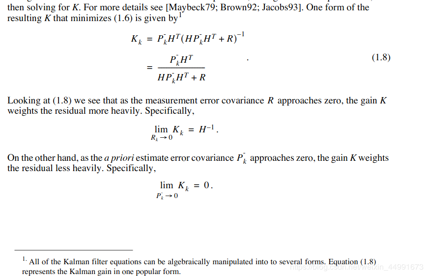
The residual reflects the discrepancy between the predicted measurement Hx^k−H\hat x_k^-Hx^k− and the actual measurementzkz_kzk . A residual of zero means that the two are in complete agreement.
KKK为卡尔曼增益。测量误差协方差趋近于0时,增益K对残差的影响更大,先验估计误差协方差趋近于零,增益K对残差的权值较小。
时间更新方程既要更新状态转移矩阵,也要更新先验误差协方差矩阵。测量更新方程先要更新卡尔曼增益K,更新状态变量,还有更新后验误差协方差矩阵。我们总是用我们的观察结果去更正我们的预测结果。
学习Michael C. Kleder 先生的代码对于卡尔曼滤波器公式的感官理解和认识有很大的帮助。
% KALMANF - updates a system state vector estimate based upon an
%           observation, using a discrete Kalman filter.
%
% Version 1.0, June 30, 2004
%
% This tutorial function was written by Michael C. Kleder
%
% INTRODUCTION
%
% Many people have heard of Kalman filtering, but regard the topic
% as mysterious. While it's true that deriving the Kalman filter and
% proving mathematically that it is "optimal" under a variety of
% circumstances can be rather intense, applying the filter to
% a basic linear system is actually very easy. This Matlab file is
% intended to demonstrate that.
%
% An excellent paper on Kalman filtering at the introductory level,
% without detailing the mathematical underpinnings, is:
% "An Introduction to the Kalman Filter"
% Greg Welch and Gary Bishop, University of North Carolina
% http://www.cs.unc.edu/~welch/kalman/kalmanIntro.html
%
% PURPOSE:
%
% The purpose of each iteration of a Kalman filter is to update
% the estimate of the state vector of a system (and the covariance
% of that vector) based upon the information in a new observation.
% The version of the Kalman filter in this function assumes that
% observations occur at fixed discrete time intervals. Also, this
% function assumes a linear system, meaning that the time evolution
% of the state vector can be calculated by means of a state transition
% matrix.
%
% USAGE:
%
% s = kalmanf(s)
%
% "s" is a "system" struct containing various fields used as input
% and output. The state estimate "x" and its covariance "P" are
% updated by the function. The other fields describe the mechanics
% of the system and are left unchanged. A calling routine may change
% these other fields as needed if state dynamics are time-dependent;
% otherwise, they should be left alone after initial values are set.
% The exceptions are the observation vectro "z" and the input control
% (or forcing function) "u." If there is an input function, then
% "u" should be set to some nonzero value by the calling routine.
%
% SYSTEM DYNAMICS:
%
% The system evolves according to the following difference equations,
% where quantities are further defined below:
%
% x = Ax + Bu + w  meaning the state vector x evolves during one time
%                  step by premultiplying by the "state transition
%                  matrix" A. There is optionally (if nonzero) an input
%                  vector u which affects the state linearly, and this
%                  linear effect on the state is represented by
%                  premultiplying by the "input matrix" B. There is also
%                  gaussian process noise w.
% z = Hx + v       meaning the observation vector z is a linear function
%                  of the state vector, and this linear relationship is
%                  represented by premultiplication by "observation
%                  matrix" H. There is also gaussian measurement
%                  noise v.
% where w ~ N(0,Q) meaning w is gaussian noise with covariance Q
%       v ~ N(0,R) meaning v is gaussian noise with covariance R
%
% VECTOR VARIABLES:
%
% s.x = state vector estimate. In the input struct, this is the
%       "a priori" state estimate (prior to the addition of the
%       information from the new observation). In the output struct,
%       this is the "a posteriori" state estimate (after the new
%       measurement information is included).
% s.z = observation vector
% s.u = input control vector, optional (defaults to zero).
%
% MATRIX VARIABLES:
%
% s.A = state transition matrix (defaults to identity).
% s.P = covariance of the state vector estimate. In the input struct,
%       this is "a priori," and in the output it is "a posteriori."
%       (required unless autoinitializing as described below).
% s.B = input matrix, optional (defaults to zero).
% s.Q = process noise covariance (defaults to zero).
% s.R = measurement noise covariance (required).
% s.H = observation matrix (defaults to identity).
%
% NORMAL OPERATION:
%
% (1) define all state definition fields: A,B,H,Q,R
% (2) define intial state estimate: x,P
% (3) obtain observation and control vectors: z,u
% (4) call the filter to obtain updated state estimate: x,P
% (5) return to step (3) and repeat
%
% INITIALIZATION:
%
% If an initial state estimate is unavailable, it can be obtained
% from the first observation as follows, provided that there are the
% same number of observable variables as state variables. This "auto-
% intitialization" is done automatically if s.x is absent or NaN.
%
% x = inv(H)*z
% P = inv(H)*R*inv(H')
%
% This is mathematically equivalent to setting the initial state estimate
% covariance to infinity.
function s = kalmanf(s)
% set defaults for absent fields:
if ~isfield(s,'x'); s.x=nan*z; end
if ~isfield(s,'P'); s.P=nan; end
if ~isfield(s,'z'); error('Observation vector missing'); end
if ~isfield(s,'u'); s.u=0; end
if ~isfield(s,'A'); s.A=eye(length(x)); end
if ~isfield(s,'B'); s.B=0; end
if ~isfield(s,'Q'); s.Q=zeros(length(x)); end
if ~isfield(s,'R'); error('Observation covariance missing'); end
if ~isfield(s,'H'); s.H=eye(length(x)); end
if isnan(s.x)
   % initialize state estimate from first observation
   if diff(size(s.H))
      error('Observation matrix must be square and invertible for state autointialization.');
   end
   s.x = inv(s.H)*s.z;
   s.P = inv(s.H)*s.R*inv(s.H');
else
   % This is the code which implements the discrete Kalman filter:
   % Prediction for state vector and covariance:
   s.x = s.A*s.x + s.B*s.u;
   s.P = s.A * s.P * s.A' + s.Q;
   % Compute Kalman gain factor:
   K = s.P*s.H'*inv(s.H*s.P*s.H'+s.R);
   % Correction based on observation:
   s.x = s.x + K*(s.z-s.H*s.x);
   s.P = s.P - K*s.H*s.P;
   % Note that the desired result, which is an improved estimate
   % of the sytem state vector x and its covariance P, was obtained
   % in only five lines of code, once the system was defined. (That's
   % how simple the discrete Kalman filter is to use.) Later,
   % we'll discuss how to deal with nonlinear systems.
end
return
测试代码如下:
% Define the system as a constant of 12 volts:
clear all
s.x = 12;
s.A = 1;
% Define a process noise (stdev) of 2 volts as the car operates:
s.Q = 2^2; % variance, hence stdev^2
% Define the voltimeter to measure the voltage itself:
s.H = 1;
% Define a measurement error (stdev) of 2 volts:
s.R = 2^2; % variance, hence stdev^2
% Do not define any system input (control) functions:
s.B = 0;
s.u = 0;
% Do not specify an initial state:
s.x = nan;
s.P = nan;
% Generate random voltages and watch the filter operate.
tru=[]; % truth voltage
for t=1:20
   tru(end+1) = randn*2+12;
   s(end).z = tru(end) + randn*2; % create a measurement
   s(end+1)=kalmanf(s(end)); % perform a Kalman filter iteration
end
figure
hold on
grid on
% plot measurement data:
hz=plot([s(1:end-1).z],'r.');
% plot a-posteriori state estimates:
hk=plot([s(2:end).x],'b-');
ht=plot(tru,'g-');
legend([hz hk ht],'observations','Kalman output','true voltage',0)
title('Automobile Voltimeter Example')
hold off
预告:扩展卡尔曼滤波器
Non-linear plant and measurement model for a simple point robot
那目前为止,我们对于卡尔曼有了浅显的认识,TA的弊端在于只能用于线性系统,很遗憾的消息是,WMRs(wheeled Mobile Robots)大多数情况下是非线性系统,为了在非线性系统中应用,我们需要进一步探索,继续向前奔跑。
假设机器人在平面上是一个点,控制输入信号是位移量,和方向偏转角度。
u(k)=[D(k),Δθ(k)]Tu(k)=[D(k),\Delta\theta(k) ]^Tu(k)=[D(k),Δθ(k)]T
在时间区域k到k+1内,WMR在移动,我们的非线性模型如下:
Φ[x(k),u(k)]=[x(k)+D(k)cos[θ(k)]y(k)+D(k)sin[θ(k)]θ(k)+Δθ(k)]\Phi[x(k),u(k)]=\begin{bmatrix}
x(k)+D(k)cos[\theta(k)] \\
y(k)+D(k)sin[\theta(k)]\\
\theta(k)+\Delta \theta(k)
\end{bmatrix}Φ[x(k),u(k)]=⎣⎡x(k)+D(k)cos[θ(k)]y(k)+D(k)sin[θ(k)]θ(k)+Δθ(k)⎦⎤
WMR 装备了传感器,可以感知到外部环境的信号浮标,我们以传感器信息对WMR 进行定位。不同的传感器有不同的定位公式,具体情况具体分析。
For example,the beacon may emit a unique sound at a known time and the robot is equipped with a microphone and listens for the sound.As long as the robot and the emitter have synchronized clocks,the distance between the beacon and the robot can be estimated.
假设信号浮标的位置(xb,yb)(x_b,y_b)(xb,yb),WMR 的测量矩阵为
h[x(k),ϵ]=[(x(k)−xb)2+(y(k)−yb)2]12h[x(k),\epsilon] =[(x(k)-x_b)^2+(y(k)-y_b)^2]^{\frac{1}{2}}h[x(k),ϵ]=[(x(k)−xb)2+(y(k)−yb)2]21
[1]An Introduction to the Kalman Filter, SIGGRAPH 2001 Course, Greg Welch and Gary Bishop
[2]详细的卡尔曼滤波器公式符号解释
[3]Computation Principles of Mobile Robotics,Cambridge University Press2000,Gregort Dudek and Michael Jenkin,Data Fusion,Page70
[4]Understanding the Covariance Matrix
最后,举起我装满白开水的保温瓶,仅以林语堂先生《论“趣”》的名言作结,与诸君共勉:)
以“名利”二字包含人生的一切活动的动机,但是还有一种知其然而不知其所以然的行为动机,叫做“趣”。
------今日更文的背景音乐,河伯《琵琶行》:)
作者:肥鼠路易