学习论文 "Edge-Labeling Graph Neural Network for Few-shot Learning"笔记
个人笔记对模型数学上的解读部分很大程度上受到这篇博客的启发与参考
NotationT=S∪QT=S \cup QT=S∪Q,support set and query set, support set SSS in each episode serves as the labeled training set
xix_ixi and yi∈{C1,...,CN}=CT⊂Cy_i \in \{C_1,...,C_N\}=C_T \subset Cyi∈{C1,...,CN}=CT⊂C: iii th input data and its label, CCC is the set of all
classes of either training or test dataset. Ctrain∩Ctest=ϕC_{train} \cap C_{test}=\phiCtrain∩Ctest=ϕ
G=(V;ξ;T)G=(V;\xi;T)G=(V;ξ;T): the graph constructed with samples from the taskTTT. V:node set; E: edge set;
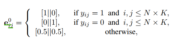
yijy_{ij}yij ground-truth edge-label, defined by the ground-truth node labels
eij={eijd}d=12∈[0,1]2\mathbf e_{ij}=\{e_{ijd}\}^2_{d=1} \in [0,1]^2eij={eijd}d=12∈[0,1]2: edge feature, representing the (normalized) strengths of the intra- and inter-class relations of the two connected nodes.
e~ijd\tilde e_{ijd}e~ijd 归一化的edge feature
fvlf^l_vfvl node feature transformation network
fe;f^;_efe; metric network
y^ij\hat y_{ij}y^ij probability that the two nodes ViV_iVi and VjV_jVj are from the same class
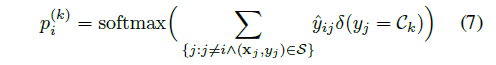
δ(yj=Ck)\delta(y_j=C_k)δ(yj=Ck) Kronecker delta function
therefore can express complex interactions among data instances. Few-shot learning algorithms have shown to require full exploitation of the relationships between a support set and a query set
So the use of GNNs can naturally have the great potential to solve the few-shot learning problem.
1. ProblemThe previous GNN approaches in few-shot learning have been mainly based on the node-labeling
framework, which implicitly models the intra-cluster similarity and inter-cluster dissimilarity
少样本学习任务,视为训练一个分类器的话,可以将此任务TTT划分为support set (输入数据和对应标签)和query set(无标签数据集)
作者采用基于元学习(meta-learning based semi-supervision)的少样本学习方法。
元学习是计算类表示形式,然后使用度量函数来度量查询样本和每个类表示形式之间的相似性。As an efficient way of meta-learning, we adopt episodic training
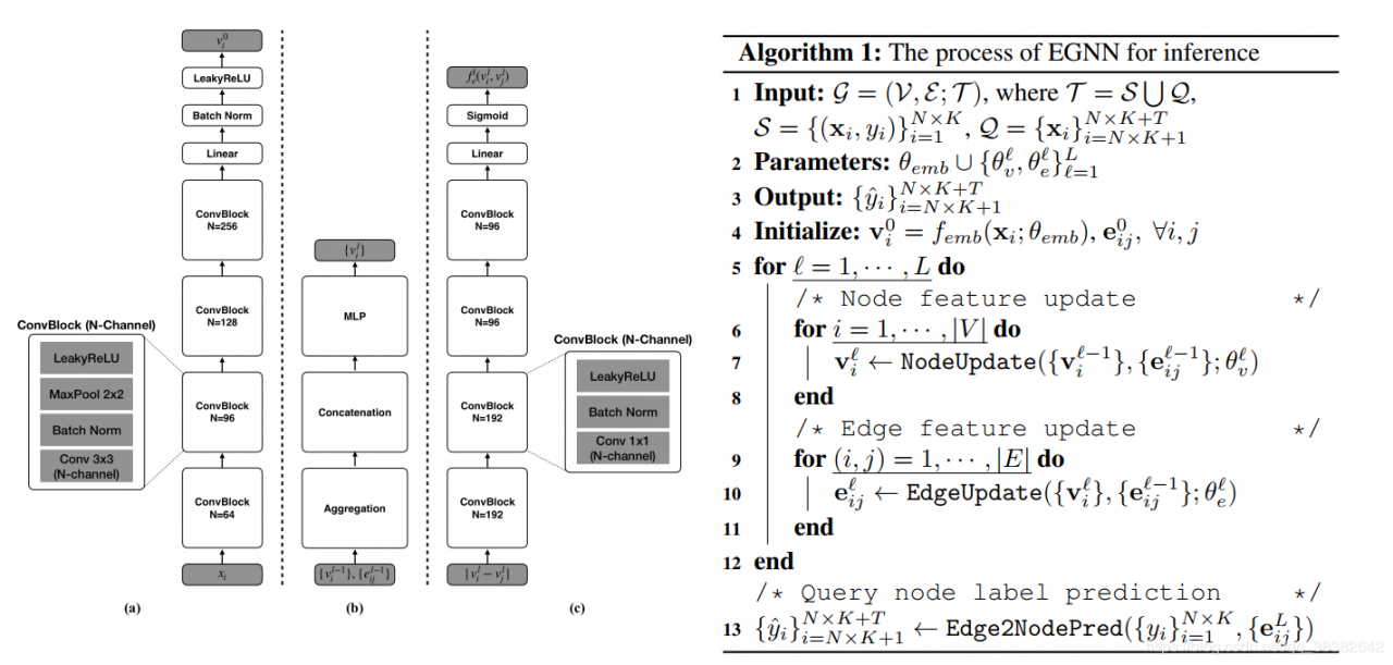
令G=(V,E;T)\mathcal{G} = (\mathcal{V},\mathcal{E};\mathcal{T})G=(V,E;T)为一个episode样本T\mathcal{T}T构建的图,∣T∣=NK+T\mathcal|{T}| = NK+T∣T∣=NK+T ; V={Vi}i=1,...,∣T∣\mathcal{V}=\{V_i\}_{i = 1,...,|\mathcal{T}|}V={Vi}i=1,...,∣T∣ 为顶点集, E={Ei}i=1,...,∣T∣\mathcal{E}=\{E_i\}_{i = 1,...,|\mathcal{T}|}E={Ei}i=1,...,∣T∣为边集。定义 边的ground true edge label

yiyiyi和yjyjyj是ground-truth node label; yijy_{ij}yij是ground-truth edge label; 如果两个node的label相同,边的label = 1
然后定义每条边为一为一个二维向量 eij={eijd}d=12∈[0,1]2e_{ij} = \{e_{ijd}\}_{d=1}^2 \in [0,1]^2eij={eijd}d=12∈[0,1]2,每一维度是一个0到1的数,和为1,表示的是类内关系和类间关系(也就是两样本类别相似性和相异性)。比如d=0d=0d=0是一个点,d=1d=1d=1是这条边对应的另一个点。
在这文章里,边的label定义eije_{ij}eij应该是不对称的,也就是eije_{ij}eij和ejie_{ji}eji 是不同的,也就是有向边。举个例子:衡量类间相似度时,eij1e_{ij1}eij1与eij2e_{ij2}eij2进行比较。衡量类内相似度时,eij1e_{ij1}eij1与eji1e_{ji1}eji1进行比较。
接下来是node feature initialized和edge feature initialized:
Node: Node features are initialized by the output of the convolutional embedding network
Edge: are initialized by edge labels
 Update
图网络包含LLL层,更新法则如下:
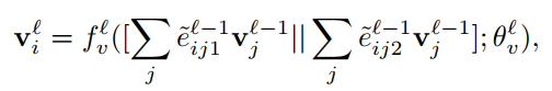
Node feature更新:和attention机制类似,用邻接节点的node信息更新当前节点。分为两部分,一部分是根据相似性提取的信息,一部分是根据相异性提取的信息,concatenate 起来
 但是,这个有着concatenate的操作相当于加权了吗?作者说与attention相似,或者可以理解为待查询的节点,与它对应的边(相当于attention的key)做键值,归一化后在feature transformation net中softmax?
看一下代码:
但是,这个有着concatenate的操作相当于加权了吗?作者说与attention相似,或者可以理解为待查询的节点,与它对应的边(相当于attention的key)做键值,归一化后在feature transformation net中softmax?
看一下代码:
class NodeUpdateNetwork(nn.Module):
    def __init__(self,
                 in_features,
                 num_features,
                 ratio=[2, 1],
                 dropout=0.0):
        super(NodeUpdateNetwork, self).__init__()
        # set size
        self.in_features = in_features
        self.num_features_list = [num_features * r for r in ratio]
        self.dropout = dropout
        # layers
        layer_list = OrderedDict()
        for l in range(len(self.num_features_list)):
            layer_list['conv{}'.format(l)] = nn.Conv2d(
                in_channels=self.num_features_list[l - 1] if l > 0 else self.in_features * 3,
                out_channels=self.num_features_list[l],
                kernel_size=1,
                bias=False)
            layer_list['norm{}'.format(l)] = nn.BatchNorm2d(num_features=self.num_features_list[l],
                                                            )
            layer_list['relu{}'.format(l)] = nn.LeakyReLU()
            if self.dropout > 0 and l == (len(self.num_features_list) - 1):
                layer_list['drop{}'.format(l)] = nn.Dropout2d(p=self.dropout)
        self.network = nn.Sequential(layer_list)
    def forward(self, node_feat, edge_feat):
        # get size
        num_tasks = node_feat.size(0)
        num_data = node_feat.size(1)
        # get eye matrix (batch_size x 2 x node_size x node_size)
        diag_mask = 1.0 - torch.eye(num_data).unsqueeze(0).unsqueeze(0).repeat(num_tasks, 2, 1, 1).to(tt.arg.device)
        # set diagonal as zero and normalize
        edge_feat = F.normalize(edge_feat * diag_mask, p=1, dim=-1)
        # compute attention and aggregate
        # 对于torch.matmul和torch.bmm,都能实现对于batch的矩阵乘法;a.squeeze(N) 就是去掉a中指定的维数为一的维度
        aggr_feat = torch.bmm(torch.cat(torch.split(edge_feat, 1, 1), 2).squeeze(1), node_feat)
        node_feat = torch.cat([node_feat, torch.cat(aggr_feat.split(num_data, 1), -1)], -1).transpose(1, 2)
        # non-linear transform
        node_feat = self.network(node_feat.unsqueeze(-1)).transpose(1, 2).squeeze(-1)
        return node_feat
输入的 in_feature :{vil−1}\{v^{l-1}_i\}{vil−1},{eijl−1}\{e^{l-1}_{ij}\}{eijl−1};
aggregation部分:
        # compute attention and aggregate
        # 对于torch.matmul和torch.bmm,都能实现对于batch的矩阵乘法;a.squeeze(N) 就是去掉a中指定的维数为一的维度
        aggr_feat = torch.bmm(torch.cat(torch.split(edge_feat, 1, 1), 2).squeeze(1), node_feat)
        node_feat = torch.cat([node_feat, torch.cat(aggr_feat.split(num_data, 1), -1)], -1).transpose(1, 2)
可以看出attention的加权在这里体现在torch.bmm的矩阵乘法上,利用边的特征edge_feat与node_feat进行了attention,所以文章说的attention应该是利用边的特征信息对节点加权。
fvlf^l_vfvl是第L层节点transform网络。在代码中的实现是将原来的feature拼接上去,另外参考了Cade博客中讲到代码中的conv2d可以改成conv1d。实际上那个卷积就是一个线性层,只不过这样处理更加方便。便于后面batchnorm和dropout对特征的每个维度做处理。
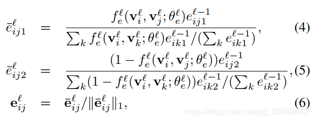
边信息的传播可以根据两个节点信息以及上一层的边信息以及和当前节点连接的其他边信息决定。
class EdgeUpdateNetwork(nn.Module):
    def __init__(self,
                 in_features,
                 num_features,
                 ratio=[2, 2, 1, 1],
                 separate_dissimilarity=False,
                 dropout=0.0):
        super(EdgeUpdateNetwork, self).__init__()
        # set size
        self.in_features = in_features
        self.num_features_list = [num_features * r for r in ratio]
        self.separate_dissimilarity = separate_dissimilarity
        self.dropout = dropout
        # layers
        layer_list = OrderedDict()
        for l in range(len(self.num_features_list)):
            # set layer
            layer_list['conv{}'.format(l)] = nn.Conv2d(in_channels=self.num_features_list[l-1] if l > 0 else self.in_features,
                                                       out_channels=self.num_features_list[l],
                                                       kernel_size=1,
                                                       bias=False)
            layer_list['norm{}'.format(l)] = nn.BatchNorm2d(num_features=self.num_features_list[l],
                                                            )
            layer_list['relu{}'.format(l)] = nn.LeakyReLU()
            if self.dropout > 0:
                layer_list['drop{}'.format(l)] = nn.Dropout2d(p=self.dropout)
        layer_list['conv_out'] = nn.Conv2d(in_channels=self.num_features_list[-1],
                                           out_channels=1,
                                           kernel_size=1)
        self.sim_network = nn.Sequential(layer_list)
        if self.separate_dissimilarity:
            # layers
            layer_list = OrderedDict()
            for l in range(len(self.num_features_list)):
                # set layer
                layer_list['conv{}'.format(l)] = nn.Conv2d(in_channels=self.num_features_list[l-1] if l > 0 else self.in_features,
                                                           out_channels=self.num_features_list[l],
                                                           kernel_size=1,
                                                           bias=False)
                layer_list['norm{}'.format(l)] = nn.BatchNorm2d(num_features=self.num_features_list[l],
                                                                )
                layer_list['relu{}'.format(l)] = nn.LeakyReLU()
                if self.dropout > 0:
                    layer_list['drop{}'.format(l)] = nn.Dropout(p=self.dropout)
            layer_list['conv_out'] = nn.Conv2d(in_channels=self.num_features_list[-1],
                                               out_channels=1,
                                               kernel_size=1)
            self.dsim_network = nn.Sequential(layer_list)
    def forward(self, node_feat, edge_feat):
        # compute abs(x_i, x_j)
        x_i = node_feat.unsqueeze(2)
        x_j = torch.transpose(x_i, 1, 2)
        x_ij = torch.abs(x_i - x_j)
        x_ij = torch.transpose(x_ij, 1, 3)# 返回输入矩阵input的转置。交换维度dim0和dim1。
        # compute similarity/dissimilarity (batch_size x feat_size x num_samples x num_samples)
        sim_val = F.sigmoid(self.sim_network(x_ij))
        if self.separate_dissimilarity:
            dsim_val = F.sigmoid(self.dsim_network(x_ij))
        else:
            dsim_val = 1.0 - sim_val
        diag_mask = 1.0 - torch.eye(node_feat.size(1)).unsqueeze(0).unsqueeze(0).repeat(node_feat.size(0), 2, 1, 1).to(tt.arg.device)
        edge_feat = edge_feat * diag_mask
        merge_sum = torch.sum(edge_feat, -1, True)  #求edge_feat各行的和
        # set diagonal as zero and normalize
        edge_feat = F.normalize(torch.cat([sim_val, dsim_val], 1) * edge_feat, p=1, dim=-1) * merge_sum
        # torch.eye 返回一个行数为node_feat.size(1)的2维张量(nxn,n=node_feat.size(1)),对角线位置全1,其它位置全0
        force_edge_feat = torch.cat((torch.eye(node_feat.size(1)).unsqueeze(0), torch.zeros(node_feat.size(1), node_feat.size(1)).unsqueeze(0)), 0).unsqueeze(0).repeat(node_feat.size(0), 1, 1, 1).to(tt.arg.device)
        edge_feat = edge_feat + force_edge_feat #把零填充上
        edge_feat = edge_feat + 1e-6
        edge_feat = edge_feat / torch.sum(edge_feat, dim=1).unsqueeze(1).repeat(1, 2, 1, 1)
        return edge_feat
其中felf^l_efel是计算相似度或不相似度的network函数:根据代码,归一化中eijl‾\overline {e^l_{ij}}eijl=F.norm(sim_val || dsim_val)×eijl\times {e^l_{ij}}×eijl其实反映的就是论文中的felf^l_efel=(sim_val || dsim_val).也就是说felf^l_efel是将similarity和dissimilarity两个联合一起表示的函数。(woc好神奇,同时表征相似和不相似)
那么(4)的式子写成∑keik1l=fel(vil,vjl)eij1l∑kfel(vil,vjl)eij1l\sum_ke^l_{ik1}=\frac{f^l_e(v^l_i,v^l_j)e^l_{ij1}}{\sum_k{f^l_e(v^l_i,v^l_j)e^l_{ij1}}}k∑eik1l=∑kfel(vil,vjl)eij1lfel(vil,vjl)eij1l∑eik1l=∑e‾ik1l(归一化)\sum e^l_{ik1}=\sum \overline e^l_{ik1}(归一化)∑eik1l=∑eik1l(归一化)
最后用有label的,去预测没有label的,方法就是利用最后输出边的相似性权重计算分类概率
整合到一起就得到算法,图模型预测的算法
 Reference
[2019][cvpr]Edge-Labeling Graph Neural Network for Few-shot Learning 笔记
作者:NERV_Dyson