Kaggle经典案例—信用卡诈骗检测的完整流程(学习笔记)

Halima ·

更新时间:2024-09-21

· 820 次阅读

本文此案例的完整流程和涉及知识

首先先看数据

import pandas as pd
import matplotlib.pyplot as plt
import numpy as np
%matplotlib inline
data = pd.read_csv("creditcard.csv")
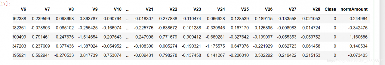
data.head()
data.shape

在这里插入图片描述
好的，它长这个样子。大致解释一下V1-V28都是一系列的指标(具体是什么不用知道)，Amount是交易金额，Class＝0表示是正常操作，而=1表示异常操作。

明确目标：检测是否异常，也就是说是一个二分类问题，接着想到用逻辑回归建模。 1.观察数据特征

Class=0的我们不妨称之为负样本，Class=1的称正样本，看一下正负样本的数量。

count_classes = pd.value_counts(data['Class'],sort = True).sort_index()
plt.figure(figsize=(10,6))
count_classes.plot(kind='bar')
plt.title("Fraud class histogram")
plt.xlabel("Class",size=20)
plt.xticks(rotation=0)
plt.ylabel("Number",size=20)

在这里插入图片描述
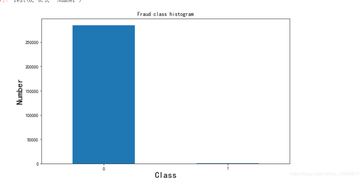
可以看出样本数据严重不均衡，样本类别不均衡将导致样本量少的分类所包含的特征过少，并很难从中提取规律。同时你的学习结果会过度拟合这种不均的结果，通俗来说就是将你的学习结果用到一组分布均匀的数据上，拟合度会很差。
那么怎么解决这个问题呢？有两种办法

采样方式选择 （1）下采样

对这个问题来说，下采样采取的方法就是取正样本中的一部分，使得正样本和负样本数量大致相同。就是让样本变得一样少

（2）过采样

相对的，过采样的做法即再生成更多的负样本数据，使得负样本和正样本一样多。就是让样本变得一样多

2.归一化处理

继续观察数据，我们可以发现Amount这一列数据的浮动差异和V1-V28数据的浮动相比差距很大。在做模型之前要保证特征之间的分布差异是差不多的，否则会对我们的模型产生误导，所以先对Amount做归一化或者标准化做法如下，使用sklearn很方便

#在这里顺便删去了Time列，因为Time列对这个问题没什么帮助
from sklearn.preprocessing import StandardScaler
data['normAmount'] = StandardScaler().fit_transform(data['Amount'].values.reshape(-1, 1))
data = data.drop(['Time','Amount'],axis=1)
data.head()

在这里插入图片描述

3.采用下采样处理数据

X = data.loc[:, data.columns != 'Class']
y = data.loc[:, data.columns == 'Class']#y=pd.DataFrame(data.loc[:,'Class'])或y=pd.DataFrame(data.Class)
number_records_fraud = len(data[data.Class == 1])
fraud_indices = np.array(data[data.Class == 1].index)
normal_indices = data[data.Class == 0].index
random_normal_indices = np.random.choice(normal_indices, number_records_fraud, replace = False)
#random.choince从所有正样本索引中随机选择负样本数量的正样本索引，replace=False表示不进行替换
random_normal_indices = np.array(random_normal_indices)
#拿出来后转成array格式
under_sample_indices = np.concatenate([fraud_indices,random_normal_indices])
#合并随机得到的正样本index和负样本
under_sample_data = data.iloc[under_sample_indices,:]
#再用index定位得到数据
X_undersample = under_sample_data.loc[:, under_sample_data.columns != 'Class']
y_undersample = under_sample_data.loc[:, under_sample_data.columns == 'Class']
#X_undersample和y_undersampl即为经过下采样处理后样本
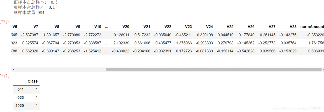
print("正样本占总样本: ", len(under_sample_data[under_sample_data.Class == 0])/len(under_sample_data))
print("负样本占总样本 ", len(under_sample_data[under_sample_data.Class == 1])/len(under_sample_data))
print("总样本数量", len(under_sample_data))
X_undersample.head(3)
y_undersample.head(3)

得到的结果：
在这里插入图片描述

交叉验证

把数据集切分成train(训练集)和test(测试集)，通常八二分，再把train等分成3个集合
在这里插入图片描述
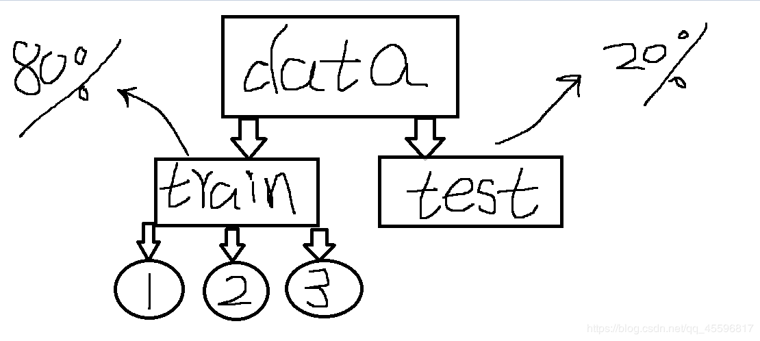
一.1+2------>3 表示用1和2建立model，用3当作验证集
二.1+3------>2 同理即1和3建model，2当作验证集
三.2+3------>1
这样做的好处如果只做一次操作，假若样本比较简单会造成模型的效率比真实值高，而如果样本存在离群值会使得模型效率比真实偏低。为了权衡两者，这样操作相当于求一个平均值，使得模型的拟合效果更理性
最后的评估效果：分别把用3，2，1的评估结果求平均值
代码实现如下：

from sklearn.model_selection import train_test_split
#sklearn中已经废弃cross_validation,将其中的内容整合到model_selection中将sklearn.cross_validation 替换为 sklearn.model_selection
X_train, X_test, y_train, y_test = train_test_split(X,y,test_size = 0.3, random_state = 0)
#随机切分，random_state=0类似设置随机数种子，test_size就是测试集比例，我这里设置为0.3即0.7训练集，0.3测试集
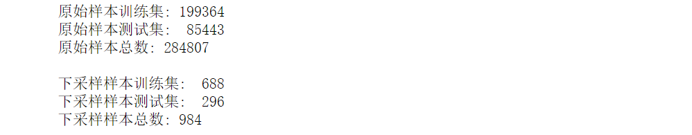
print("原始样本训练集:", len(X_train))
print("原始样本测试集: ", len(X_test))
print("原始样本总数:", len(X_train)+len(X_test))
#对下采样数据也进行切分
X_train_undersample, X_test_undersample, y_train_undersample, y_test_undersample = train_test_split(X_undersample,y_undersample
                                                                                                   ,test_size = 0.3
                                                                                                   ,random_state = 0)
print("")
print("下采样样本训练集: ", len(X_train_undersample))
print("下采样样本测试集: ", len(X_test_undersample))
print("下采样样本总数:", len(X_train_undersample)+len(X_test_undersample))

在这里插入图片描述

#Recall = TP/(TP+FN)通过召回率评估模型
#TP（true positives）FP（false positives）FN（false negatives）TN（true negatives）
from sklearn.linear_model import LogisticRegression#引入逻辑回归模型
from sklearn.model_selection import KFold, cross_val_score
#KFlod指做几倍的交叉验证，cross_val_score为交叉验证评估结果
from sklearn.metrics import confusion_matrix,recall_score,classification_report
#confusion_matrix混淆矩阵

关于Recall的解释这篇文章讲的很清楚

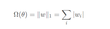
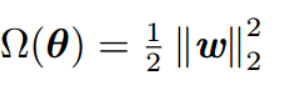
正则化惩罚项

假设有两组权重参数A和B，它们的RECALL值相同，但是A这组的方差远大于B，那么A比B更容易出现**过拟合(在训练集效果良好但在测试集变现差)**的情况。所以为了得到B这样的模型，引入正则化惩罚项。即把目标函数变成 损失函数+正则化惩罚项
正则化惩罚项分两种：
L1：
在这里插入图片描述
L2:

def printing_Kfold_scores(x_train_data,y_train_data):#fold.split(y_train_data)
c_param_range = [0.01,0.1,1,10,100]
#正则化惩罚力度候选
results_table = pd.DataFrame(index = range(len(c_param_range),2), columns = ['C_parameter','Mean recall score'])
results_table['C_parameter'] = c_param_range
# the k-fold will give 2 lists: train_indices = indices[0], test_indices = indices[1]
j = 0
for c_param in c_param_range:#找出最合适的正则化惩罚力度
    print('-------------------------------------------')
    print('C parameter: ', c_param)
    print('-------------------------------------------')
    print('')
    recall_accs = []
    for iteration, indices in enumerate(fold.split(y_train_data),start=1):
        lr = LogisticRegression(C = c_param, penalty = 'l1',solver='liblinear')
        #C是惩罚力度，penalty是选择l1还是l2惩罚，solver可选参数:{‘liblinear’, ‘sag’, ‘saga’,‘newton-cg’, ‘lbfgs’}
        lr.fit(x_train_data.iloc[indices[0],:],y_train_data.iloc[indices[0],:].values.ravel())
        #lr.fit:训练lr模型,传入dataframe的X和转变成一行的y
        y_pred_undersample = lr.predict(x_train_data.iloc[indices[1],:].values)
        #lr.predict:用验证样本集进行预测
        recall_acc = recall_score(y_train_data.iloc[indices[1],:].values,y_pred_undersample)
        #recall_score：传入结果集，和predict的结果得到评估结果
        recall_accs.append(recall_acc)
        print('Iteration ', iteration,': recall score = ', recall_acc)
    results_table.loc[j,'Mean recall score'] = np.mean(recall_accs)
    j += 1
    print('')
    print('Mean recall score ', np.mean(recall_accs))
    print('')
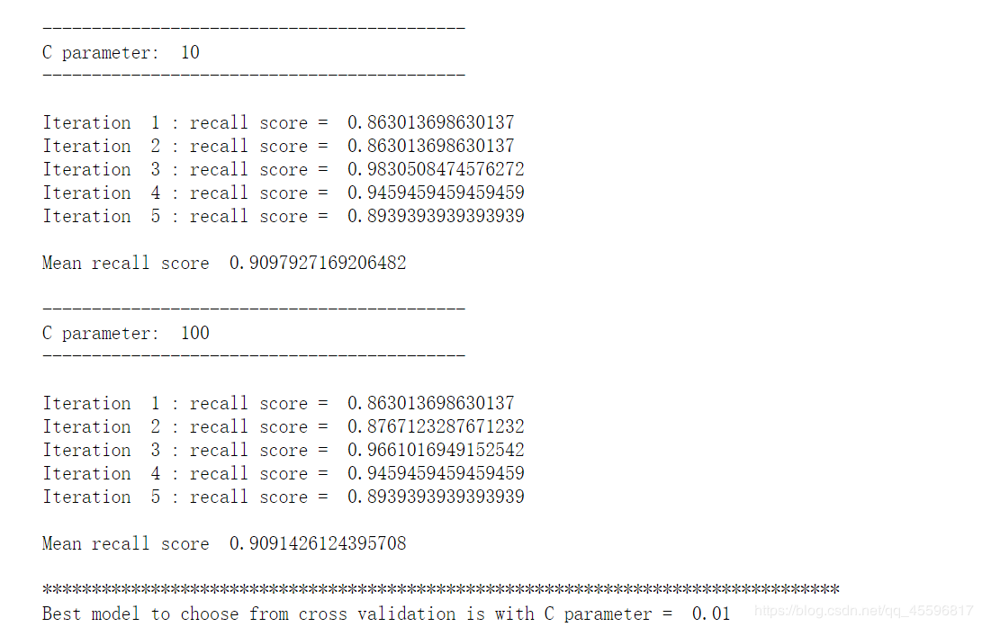
best_c = results_table.loc[np.argmax(np.array(results_table['Mean recall score']))]['C_parameter']
print('*********************************************************************************')
print('Best model to choose from cross validation is with C parameter = ', best_c)
print('*********************************************************************************')
return best_c
best_c = printing_Kfold_scores(X_train_undersample,y_train_undersample)

具体迭代过程就不看了，感兴趣的可以复制过去跑一下，最终得到结果如下
在这里插入图片描述
用下采样训练的模型画混淆矩阵

def plot_confusion_matrix(cm, classes,
                          title='Confusion matrix',
                          cmap=plt.cm.Blues):
    plt.imshow(cm, interpolation='nearest', cmap=cmap,aspect='auto')
    plt.title(title)
    plt.colorbar()
    tick_marks = np.arange(len(classes))
    plt.xticks(tick_marks, classes, rotation=0)
    plt.yticks(tick_marks, classes)
    thresh = cm.max() / 2.
    for i, j in itertools.product(range(cm.shape[0]), range(cm.shape[1])):
        plt.text(j, i, cm[i, j],
                 horizontalalignment="center",
                 color="white" if cm[i, j] > thresh else "black")
    plt.tight_layout()
    plt.ylabel('True label')
    plt.xlabel('Predicted label')
    import itertools
lr = LogisticRegression(C = best_c, penalty = 'l2')
lr.fit(X_train_undersample,y_train_undersample.values.ravel())
y_pred_undersample = lr.predict(X_test_undersample.values)
cnf_matrix = confusion_matrix(y_test_undersample,y_pred_undersample)
np.set_printoptions(precision=2)
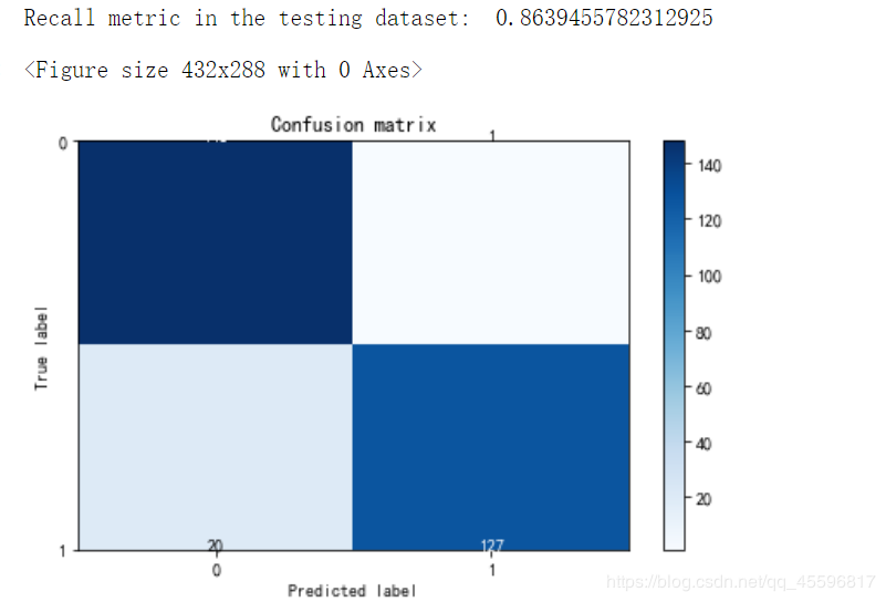
print("Recall metric in the testing dataset: ", cnf_matrix[1,1]/(cnf_matrix[1,0]+cnf_matrix[1,1]))
class_names = [0,1]
plt.figure()
plot_confusion_matrix(cnf_matrix
                      , classes=class_names
                      , title='Confusion matrix')
plt.show()

这个是用模型拟合下采样测试集结果，我这个由于matplotlib库版本问题数据有点错位。
不过可以看出TP=138,TN=9,FP=9,FN看不太清不过和TP差不多
RECALL值有0.863
在这里插入图片描述
再用模型拟合原数据的测试集画混淆矩阵

lr = LogisticRegression(C = best_c, penalty = 'l1',solver='liblinear')
lr.fit(X_train_undersample,y_train_undersample.values.ravel())
y_pred = lr.predict(X_test.values)
# Compute confusion matrix
cnf_matrix = confusion_matrix(y_test,y_pred)
np.set_printoptions(precision=2)
print("Recall metric in the testing dataset: ", cnf_matrix[1,1]/(cnf_matrix[1,0]+cnf_matrix[1,1]))
# Plot non-normalized confusion matrix
class_names = [0,1]
plt.figure()
plot_confusion_matrix(cnf_matrix
                      , classes=class_names
                      , title='Confusion matrix')
plt.show()

在这里插入图片描述
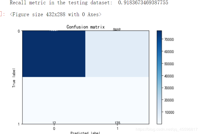
RECALL值满意需求，但是还是存在问题。FP这类有8000多个，也就是说** 原本正常被当初异常即“误杀”的样本有8000多个，会使得精度降低**

4.对比下采样和直接拿原始数据训练模型

best_c = printing_Kfold_scores(X_train,y_train)
#用原始数据训练，找最佳的正则化惩罚项
lr = LogisticRegression(C = best_c, penalty = 'l2')
lr.fit(X_train,y_train.values.ravel())
y_pred_undersample = lr.predict(X_test.values)
# Compute confusion matrix
cnf_matrix = confusion_matrix(y_test,y_pred_undersample)
np.set_printoptions(precision=2)
print("Recall metric in the testing dataset: ", cnf_matrix[1,1]/(cnf_matrix[1,0]+cnf_matrix[1,1]))
# Plot non-normalized confusion matrix
class_names = [0,1]
plt.figure()
plot_confusion_matrix(cnf_matrix
                      , classes=class_names
                      , title='Confusion matrix')
plt.show()

可以看到结果很不理想，RECALL值很低，所以样本不均的情况下不做处理做出的模型通常很差。
在这里插入图片描述

5.逻辑回归阈值对结果的影响

lr = LogisticRegression(C = 0.01, penalty = 'l1',solver='liblinear')
lr.fit(X_train_undersample,y_train_undersample.values.ravel())
y_pred_undersample_proba = lr.predict_proba(X_test_undersample.values)
#lr.predict_proba 预测出一个概率值
thresholds = [0.1,0.2,0.3,0.4,0.5,0.6,0.7,0.8,0.9]
#指定一系列阈值
plt.figure(figsize=(12,10))
j = 1
for i in thresholds:
    y_test_predictions_high_recall = y_pred_undersample_proba[:,1] > i
    plt.subplot(3,3,j)
    j += 1
    cnf_matrix = confusion_matrix(y_test_undersample,y_test_predictions_high_recall)
    np.set_printoptions(precision=2)
    print("Recall metric in the testing dataset: ", cnf_matrix[1,1]/(cnf_matrix[1,0]+cnf_matrix[1,1]))
    # Plot non-normalized confusion matrix
    class_names = [0,1]
    plot_confusion_matrix(cnf_matrix, classes=class_names,title='Threshold >= %s'%i) 
#右上角是误杀的，左下角是没被揪出来的异常

原来默认是概率大于0.5就认为是异常，这个阈值可以自己设定，阈值越大即表示越严格。
可以看出不同阈值对结果的影响，RECALL是一个递减的过程，精度逐渐增大

在这里插入图片描述
所以阈值的选取通常根据实际要求合理选取，好的模型RECALL和精度都要保证尽量高。