线性回归中,MGD、BGD与MBGD对比研究(三)——以鸢尾花数据集为例
上一次,写了MGD、SGD、MBGD的代码实现,现在,我们来康康实例
我们以大名鼎鼎的鸢尾花数据集为例:
https://archive.ics.uci.edu/ml/machine-learning-databases/iris/
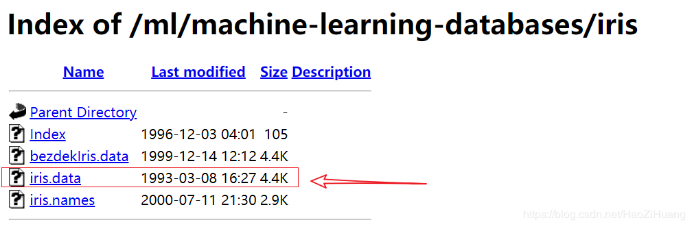
下载这个iris.data即可
将其置于当前工作文件夹即可
先导入需要的库:
import numpy as np
import pandas as pd
import random
然后将我们上一次写的函数copy过来:
def MGD_train(X, y, alpha=0.0001, maxIter=1000, theta_old=None):
    '''
    MGD训练线性回归
    传入:
        X       :  已知数据
        y       :  标签
        alpha   :  学习率
        maxIter :  总迭代次数
    返回:
        theta : 权重参数
    '''
    # 初始化权重参数
    theta = np.ones(shape=(X.shape[1],))
    if not theta_old is None:
        # 假装是断点续训练
        theta = theta_old.copy()
    for i in range(maxIter):
        # 预测
        y_pred = np.sum(X * theta, axis=1)
        # 全部数据得到的梯度
        gradient = np.average((y - y_pred).reshape(-1, 1) * X, axis=0)
        # 更新学习率
        theta += alpha * gradient
    return theta
def SGD_train(X, y, alpha=0.0001, maxIter=1000, theta_old=None):
    '''
    SGD训练线性回归
    传入:
        X       :  已知数据
        y       :  标签
        alpha   :  学习率
        maxIter :  总迭代次数
    返回:
        theta : 权重参数
    '''
    # 初始化权重参数
    theta = np.ones(shape=(X.shape[1],))
    if not theta_old is None:
        # 假装是断点续训练
        theta = theta_old.copy()
    # 数据数量
    data_length = X.shape[0]
    for i in range(maxIter):
        # 随机选择一个数据
        index = np.random.randint(0, data_length)
        # 预测
        y_pred = np.sum(X[index, :] * theta)
        # 一条数据得到的梯度
        gradient = (y[index] - y_pred) * X[index, :]
        # 更新学习率
        theta += alpha * gradient
    return theta
def MBGD_train(X, y, alpha=0.0001, maxIter=1000, batch_size=10, theta_old=None):
    '''
    MBGD训练线性回归
    传入:
        X          :  已知数据
        y          :  标签
        alpha      :  学习率
        maxIter    :  总迭代次数
        batch_size :  没一轮喂入的数据数
    返回:
        theta : 权重参数
    '''
    # 初始化权重参数
    theta = np.ones(shape=(X.shape[1],))
    if not theta_old is None:
        # 假装是断点续训练
        theta = theta_old.copy()
    # 所有数据的集合
    all_data = np.concatenate([X, y.reshape(-1, 1)], axis=1)
    for i in range(maxIter):
        # 从全部数据里选 batch_size 个 item
        X_batch_size = np.array(random.choices(all_data, k=batch_size))
        # 重新给 X, y 赋值
        X_new = X_batch_size[:, :-1]
        y_new = X_batch_size[:, -1]
        # 将数据喂入, 更新 theta
        theta = MGD_train(X_new, y_new, alpha=0.0001, maxIter=1, theta_old=theta)
    return theta
def GD_predict(X, theta):
    '''
    用于预测的函数
    传入:
        X     : 数据
        theta : 权重
    返回:
        y_pred: 预测向量
    '''
    y_pred = np.sum(theta * X, axis=1)
    # 实数域空间 -> 离散三值空间, 则需要四舍五入
    y_pred = (y_pred + 0.5).astype(int)
    return y_pred
def calc_accuracy(y, y_pred):
    '''
    计算准确率
    传入:
        y        : 标签
        y_pred   : 预测值
    返回:
        accuracy : 准确率
    '''
    return np.average(y == y_pred)*100
以上是需要用到的函数
# 读取数据
iris_raw_data = pd.read_csv('./iris.data', names  =['sepal length', 'sepal width', 'petal length', 'petal width', 'class'])
# 将三种类型映射成整数
Iris_dir = {'Iris-setosa': 1, 'Iris-versicolor': 2, 'Iris-virginica': 3}
iris_raw_data['class'] = iris_raw_data['class'].apply(lambda x:Iris_dir[x])
# 训练数据 X
iris_data = iris_raw_data.values[:, :-1]
# 标签 y
y = iris_raw_data.values[:, -1]
# 用MGD训练的参数
start = time.time()
theta_MGD = MGD_train(iris_data, y)
run_time = time.time() - start
y_pred_MGD = GD_predict(iris_data, theta_MGD)
print("MGD训练1000轮得到的准确率{:.2f}% 运行时间是{:.2f}s".format(calc_accuracy(y, y_pred_MGD), run_time))
# 用SGD训练的参数
start = time.time()
theta_SGD = SGD_train(iris_data, y)
run_time = time.time() - start
y_pred_SGD = GD_predict(iris_data, theta_SGD)
print("SGD训练1000轮得到的准确率{:.2f}% 运行时间是{:.2f}s".format(calc_accuracy(y, y_pred_SGD), run_time))
# 用MBGD训练的参数
start = time.time()
theta_MBGD = MBGD_train(iris_data, y)
run_time = time.time() - start
y_pred_MBGD = GD_predict(iris_data, theta_MBGD)
print("MBGD训练1000轮得到的准确率{:.2f}% 运行时间是{:.2f}s".format(calc_accuracy(y, y_pred_MBGD), run_time))
运行一下:
MGD训练1000轮得到的准确率92.67% 运行时间是0.02s
SGD训练1000轮得到的准确率93.33% 运行时间是0.01s
MBGD训练1000轮得到的准确率92.67% 运行时间是0.05s
(你得到的结果准确率可能有些不同,因为在SGD和MBGD中,有随机部分)
另外,运行时间和我们预想的有较大差异,尤其是MBGD竟然时间最长,是因为笔者在实现代码时,有这样一句话:
X_batch_size = np.array(random.choices(all_data, k=batch_size))
这个随机过程消耗了大量时间
下一篇,我们试一试,可视化loss——tensorboard
作者:Ryan Huang
相关文章
Oprah
2020-06-20
Brigitte
2021-08-06
Quirita
2020-01-27
Peren
2020-12-22
Grizelda
2023-07-20
Penny
2023-07-20
Janna
2023-07-20
Ophelia
2023-07-21
Crystal
2023-07-21
Laila
2023-07-21
Aine
2023-07-21
Bliss
2023-07-21
Lillian
2023-07-21
Tertia
2023-07-21
Olive
2023-07-21
Angie
2023-07-21
Nora
2023-07-24