python实现梯度下降求解逻辑回归
本文实例为大家分享了python实现梯度下降求解逻辑回归的具体代码,供大家参考,具体内容如下
对比线性回归理解逻辑回归,主要包含回归函数,似然函数,梯度下降求解及代码实现
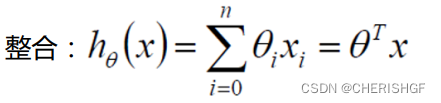
线性回归 1.线性回归函数
似然函数的定义:给定联合样本值X下关于(未知)参数
的函数
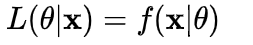

似然函数:什么样的参数跟我们的数据组合后恰好是真实值
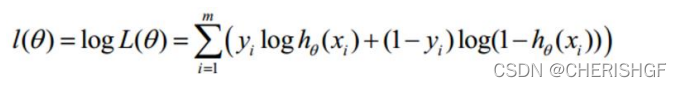
2.线性回归似然函数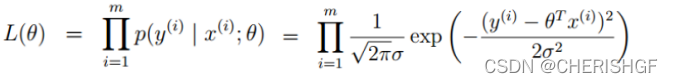
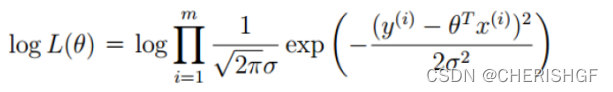
对数似然:
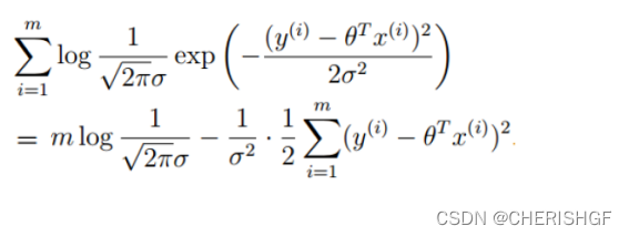
(误差的表达式,我们的目的就是使得真实值与预测值之前的误差最小)

(导数为0取得极值,得到函数的参数)
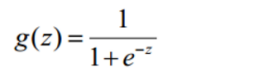
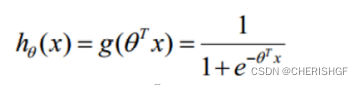
逻辑回归逻辑回归是在线性回归的结果外加一层Sigmoid函数
前提数据服从伯努利分布
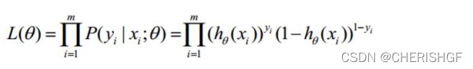
对数似然:
引入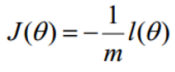 转变为梯度下降任务,逻辑回归目标函数
我的理解就是求导更新参数,达到一定条件后停止,得到近似最优解
代码实现Sigmoid函数
def sigmoid(z):
return 1 / (1 + np.exp(-z))
预测函数
def model(X, theta):
    return sigmoid(np.dot(X, theta.T))
目标函数
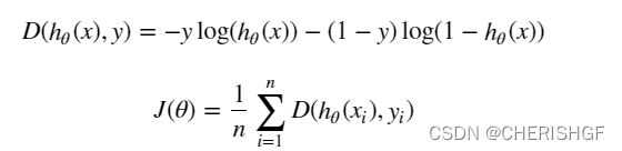
def cost(X, y, theta):
left = np.multiply(-y, np.log(model(X, theta)))
right = np.multiply(1 - y, np.log(1 - model(X, theta)))
return np.sum(left - right) / (len(X))
梯度
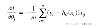
def gradient(X, y, theta):
grad = np.zeros(theta.shape)
error = (model(X, theta)- y).ravel()
for j in range(len(theta.ravel())): #for each parmeter
term = np.multiply(error, X[:,j])
grad[0, j] = np.sum(term) / len(X)
return grad
梯度下降停止策略
STOP_ITER = 0
STOP_COST = 1
STOP_GRAD = 2
def stopCriterion(type, value, threshold):
    # 设定三种不同的停止策略
    if type == STOP_ITER:  # 设定迭代次数
        return value > threshold
    elif type == STOP_COST:  # 根据损失值停止
        return abs(value[-1] - value[-2]) < threshold
    elif type == STOP_GRAD:  # 根据梯度变化停止
        return np.linalg.norm(value) < threshold
样本重新洗牌
import numpy.random
#洗牌
def shuffleData(data):
    np.random.shuffle(data)
    cols = data.shape[1]
    X = data[:, 0:cols-1]
    y = data[:, cols-1:]
    return X, y
梯度下降求解
def descent(data, theta, batchSize, stopType, thresh, alpha):
    # 梯度下降求解
    init_time = time.time()
    i = 0  # 迭代次数
    k = 0  # batch
    X, y = shuffleData(data)
    grad = np.zeros(theta.shape)  # 计算的梯度
    costs = [cost(X, y, theta)]  # 损失值
    while True:
        grad = gradient(X[k:k + batchSize], y[k:k + batchSize], theta)
        k += batchSize  # 取batch数量个数据
        if k >= n:
            k = 0
            X, y = shuffleData(data)  # 重新洗牌
        theta = theta - alpha * grad  # 参数更新
        costs.append(cost(X, y, theta))  # 计算新的损失
        i += 1
        if stopType == STOP_ITER:
            value = i
        elif stopType == STOP_COST:
            value = costs
        elif stopType == STOP_GRAD:
            value = grad
        if stopCriterion(stopType, value, thresh): break
    return theta, i - 1, costs, grad, time.time() - init_time
完整代码
import numpy as np
import pandas as pd
import matplotlib.pyplot as plt
import os
import numpy.random
import time
def sigmoid(z):
    return 1 / (1 + np.exp(-z))
def model(X, theta):
    return sigmoid(np.dot(X, theta.T))
def cost(X, y, theta):
    left = np.multiply(-y, np.log(model(X, theta)))
    right = np.multiply(1 - y, np.log(1 - model(X, theta)))
    return np.sum(left - right) / (len(X))
def gradient(X, y, theta):
    grad = np.zeros(theta.shape)
    error = (model(X, theta) - y).ravel()
    for j in range(len(theta.ravel())):  # for each parmeter
        term = np.multiply(error, X[:, j])
        grad[0, j] = np.sum(term) / len(X)
    return grad
STOP_ITER = 0
STOP_COST = 1
STOP_GRAD = 2
def stopCriterion(type, value, threshold):
    # 设定三种不同的停止策略
    if type == STOP_ITER:  # 设定迭代次数
        return value > threshold
    elif type == STOP_COST:  # 根据损失值停止
        return abs(value[-1] - value[-2]) < threshold
    elif type == STOP_GRAD:  # 根据梯度变化停止
        return np.linalg.norm(value) < threshold
# 洗牌
def shuffleData(data):
    np.random.shuffle(data)
    cols = data.shape[1]
    X = data[:, 0:cols - 1]
    y = data[:, cols - 1:]
    return X, y
def descent(data, theta, batchSize, stopType, thresh, alpha):
    # 梯度下降求解
    init_time = time.time()
    i = 0  # 迭代次数
    k = 0  # batch
    X, y = shuffleData(data)
    grad = np.zeros(theta.shape)  # 计算的梯度
    costs = [cost(X, y, theta)]  # 损失值
    while True:
        grad = gradient(X[k:k + batchSize], y[k:k + batchSize], theta)
        k += batchSize  # 取batch数量个数据
        if k >= n:
            k = 0
            X, y = shuffleData(data)  # 重新洗牌
        theta = theta - alpha * grad  # 参数更新
        costs.append(cost(X, y, theta))  # 计算新的损失
        i += 1
        if stopType == STOP_ITER:
            value = i
        elif stopType == STOP_COST:
            value = costs
        elif stopType == STOP_GRAD:
            value = grad
        if stopCriterion(stopType, value, thresh): break
    return theta, i - 1, costs, grad, time.time() - init_time
def runExpe(data, theta, batchSize, stopType, thresh, alpha):
    # import pdb
    # pdb.set_trace()
    theta, iter, costs, grad, dur = descent(data, theta, batchSize, stopType, thresh, alpha)
    name = "Original" if (data[:, 1] > 2).sum() > 1 else "Scaled"
    name += " data - learning rate: {} - ".format(alpha)
    if batchSize == n:
        strDescType = "Gradient"  # 批量梯度下降
    elif batchSize == 1:
        strDescType = "Stochastic"  # 随机梯度下降
    else:
        strDescType = "Mini-batch ({})".format(batchSize)  # 小批量梯度下降
    name += strDescType + " descent - Stop: "
    if stopType == STOP_ITER:
        strStop = "{} iterations".format(thresh)
    elif stopType == STOP_COST:
        strStop = "costs change < {}".format(thresh)
    else:
        strStop = "gradient norm < {}".format(thresh)
    name += strStop
    print("***{}\nTheta: {} - Iter: {} - Last cost: {:03.2f} - Duration: {:03.2f}s".format(
        name, theta, iter, costs[-1], dur))
    fig, ax = plt.subplots(figsize=(12, 4))
    ax.plot(np.arange(len(costs)), costs, 'r')
    ax.set_xlabel('Iterations')
    ax.set_ylabel('Cost')
    ax.set_title(name.upper() + ' - Error vs. Iteration')
    return theta
path = 'data' + os.sep + 'LogiReg_data.txt'
pdData = pd.read_csv(path, header=None, names=['Exam 1', 'Exam 2', 'Admitted'])
positive = pdData[pdData['Admitted'] == 1]
negative = pdData[pdData['Admitted'] == 0]
# 画图观察样本情况
fig, ax = plt.subplots(figsize=(10, 5))
ax.scatter(positive['Exam 1'], positive['Exam 2'], s=30, c='b', marker='o', label='Admitted')
ax.scatter(negative['Exam 1'], negative['Exam 2'], s=30, c='r', marker='x', label='Not Admitted')
ax.legend()
ax.set_xlabel('Exam 1 Score')
ax.set_ylabel('Exam 2 Score')
pdData.insert(0, 'Ones', 1)
# 划分训练数据与标签
orig_data = pdData.values
cols = orig_data.shape[1]
X = orig_data[:, 0:cols - 1]
y = orig_data[:, cols - 1:cols]
# 设置初始参数0
theta = np.zeros([1, 3])
# 选择的梯度下降方法是基于所有样本的
n = 100
runExpe(orig_data, theta, n, STOP_ITER, thresh=5000, alpha=0.000001)
runExpe(orig_data, theta, n, STOP_COST, thresh=0.000001, alpha=0.001)
runExpe(orig_data, theta, n, STOP_GRAD, thresh=0.05, alpha=0.001)
runExpe(orig_data, theta, 1, STOP_ITER, thresh=5000, alpha=0.001)
runExpe(orig_data, theta, 1, STOP_ITER, thresh=15000, alpha=0.000002)
runExpe(orig_data, theta, 16, STOP_ITER, thresh=15000, alpha=0.001)
from sklearn import preprocessing as pp
# 数据预处理
scaled_data = orig_data.copy()
scaled_data[:, 1:3] = pp.scale(orig_data[:, 1:3])
runExpe(scaled_data, theta, n, STOP_ITER, thresh=5000, alpha=0.001)
runExpe(scaled_data, theta, n, STOP_GRAD, thresh=0.02, alpha=0.001)
theta = runExpe(scaled_data, theta, 1, STOP_GRAD, thresh=0.002 / 5, alpha=0.001)
runExpe(scaled_data, theta, 16, STOP_GRAD, thresh=0.002 * 2, alpha=0.001)
# 设定阈值
def predict(X, theta):
    return [1 if x >= 0.5 else 0 for x in model(X, theta)]
# 计算精度
scaled_X = scaled_data[:, :3]
y = scaled_data[:, 3]
predictions = predict(scaled_X, theta)
correct = [1 if ((a == 1 and b == 1) or (a == 0 and b == 0)) else 0 for (a, b) in zip(predictions, y)]
accuracy = (sum(map(int, correct)) % len(correct))
print('accuracy = {0}%'.format(accuracy))
逻辑回归的优缺点
优点
形式简单,模型的可解释性非常好。从特征的权重可以看到不同的特征对最后结果的影响,某个特征的权重值比较高,那么这个特征最后对结果的影响会比较大。
模型效果不错。在工程上是可以接受的(作为baseline),如果特征工程做的好,效果不会太差,并且特征工程可以大家并行开发,大大加快开发的速度。
训练速度较快。分类的时候,计算量仅仅只和特征的数目相关。并且逻辑回归的分布式优化sgd发展比较成熟,训练的速度可以通过堆机器进一步提高,这样我们可以在短时间内迭代好几个版本的模型。
资源占用小,尤其是内存。因为只需要存储各个维度的特征值。
方便输出结果调整。逻辑回归可以很方便的得到最后的分类结果,因为输出的是每个样本的概率分数,我们可以很容易的对这些概率分数进行cutoff,也就是划分阈值(大于某个阈值的是一类,小于某个阈值的是一类)。
缺点准确率并不是很高。因为形式非常的简单(非常类似线性模型),很难去拟合数据的真实分布。
很难处理数据不平衡的问题。举个例子:如果我们对于一个正负样本非常不平衡的问题比如正负样本比 10000:1.我们把所有样本都预测为正也能使损失函数的值比较小。但是作为一个分类器,它对正负样本的区分能力不会很好。
处理非线性数据较麻烦。逻辑回归在不引入其他方法的情况下,只能处理线性可分的数据,或者进一步说,处理二分类的问题 。
逻辑回归本身无法筛选特征。有时候,我们会用gbdt来筛选特征,然后再上逻辑回归。