从零基础入门Tensorflow2.0 ----二、5.1 超参数搜索

Phaedra ·

更新时间:2024-09-21

· 974 次阅读

every blog every motto: Love is not a maybe thing. You know when you love someone.

0. 前言

手动实现超参数搜索，下一节我们将讲利用skleran实现

1. 代码部分 1. 导入模块

import matplotlib as mpl
import matplotlib.pyplot as plt
%matplotlib inline
import numpy as np
import sklearn
import pandas as pd
import os
import sys
import time
import tensorflow as tf
from tensorflow import keras
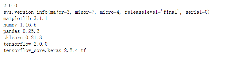
print(tf.__version__)
print(sys.version_info)
for module in mpl,np,pd,sklearn,tf,keras:
    print(module.__name__,module.__version__)

在这里插入图片描述

2. 读取数据

from sklearn.datasets import fetch_california_housing
# 房价预测
housing = fetch_california_housing()
print(housing.DESCR)
print(housing.data.shape)
print(housing.target.shape)

3. 划分样本

# 划分样本
from sklearn.model_selection import train_test_split
x_train_all,x_test,y_train_all,y_test = train_test_split(housing.data,housing.target,random_state=7)
x_train,x_valid,y_train,y_valid = train_test_split(x_train_all,y_train_all,random_state=11)
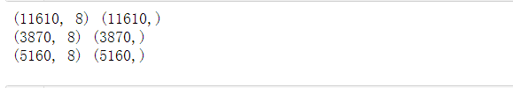
print(x_train.shape,y_train.shape)
print(x_valid.shape,y_valid.shape)
print(x_test.shape,y_test.shape)

在这里插入图片描述

4. 数据归一化

# 归一化
from sklearn.preprocessing import StandardScaler
scaler = StandardScaler()
x_train_scaled = scaler.fit_transform(x_train)
x_valid_scaled = scaler.transform(x_valid)
x_test_scaled = scaler.transform(x_test)

5. 构建模型（超参数搜索实现）

# 超参数搜索
# learn_rate : [1e-4,3e-4,1e-3,3e-3,1e-2,3e-2]
learning_rates = [1e-4,3e-4,1e-3,3e-3,1e-2,2e-2]
histories = []
for lr in learning_rates:
    # 搭建模型
    model = keras.models.Sequential([
        keras.layers.Dense(30,activation='relu',input_shape=x_train.shape[1:]),
        keras.layers.Dense(1),
    ])
    optimizer = keras.optimizers.SGD(lr)
    # 编译
    model.compile(loss='mean_squared_error',optimizer=optimizer)
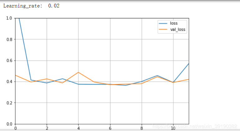
    # 回调函数
    callbacks = [keras.callbacks.EarlyStopping(patience=5,min_delta=1e-3)]
    #训练
    history = model.fit(x_train_scaled,y_train,validation_data=(x_valid_scaled,y_valid),epochs=100,callbacks=callbacks)
    histories.append(history)

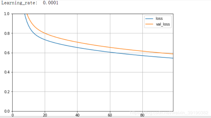
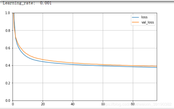
6. 学习曲线

# 学习曲线
def plot_learning_curves(history):
    pd.DataFrame(history.history).plot(figsize=(8,5))
    plt.grid(True)
    plt.gca().set_ylim(0,1)
    plt.show()
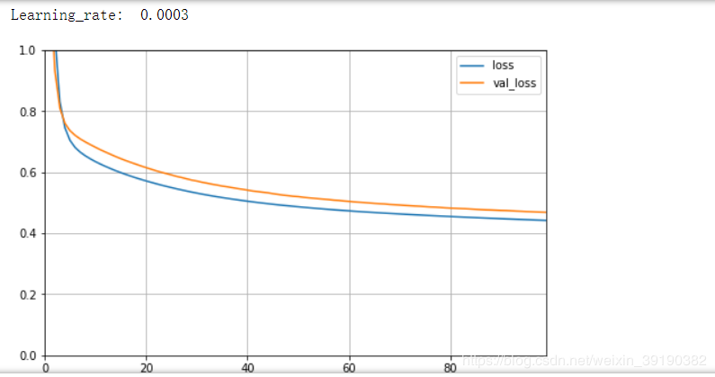
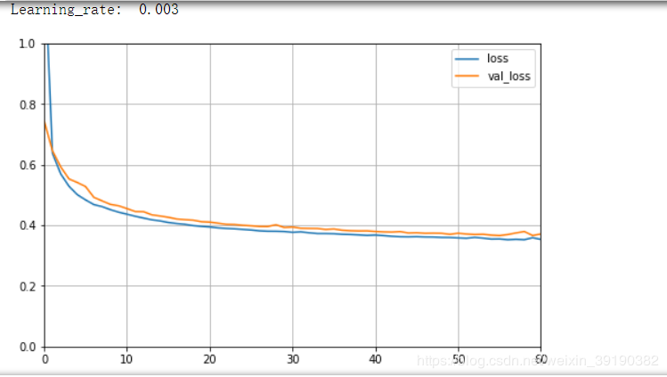
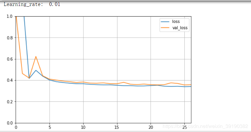
for lr,history in zip(learning_rates,histories):
    print("Learning_rate: ",lr)
    plot_learning_curves(history)

在这里插入图片描述