kaggle入门赛TOP%7:泰坦尼克号(1.数据分析,特征处理)基于百度aistudio平台
目前排名1420/19000
数据可视化分析
```python
#保存一下数据,防止丢失
trainSet.to_csv('work/trainSet1.csv',index=0)
testSet.to_csv('work/testSet1.csv',index=0)
数据终于处理完了,下面进行建模预测
建模预测在下一篇帖子:
https://blog.csdn.net/QianLong_/article/details/105780130
# 查看当前挂载的数据集目录, 该目录下的变更重启环境后会自动还原
# View dataset directory. This directory will be recovered automatically after resetting environment.
!ls /home/aistudio/data
data31483
# 查看工作区文件, 该目录下的变更将会持久保存. 请及时清理不必要的文件, 避免加载过慢.
# View personal work directory. All changes under this directory will be kept even after reset. Please clean unnecessary files in time to speed up environment loading.
!ls /home/aistudio/work
gender_submission.csv test.csv train.csv
# 如果需要进行持久化安装, 需要使用持久化路径, 如下方代码示例:
# If a persistence installation is required, you need to use the persistence path as the following:
!mkdir /home/aistudio/external-libraries
!pip install seaborn -t /home/aistudio/external-libraries
Looking in indexes: https://pypi.mirrors.ustc.edu.cn/simple/
Collecting seaborn
[?25l  Downloading https://mirrors.tuna.tsinghua.edu.cn/pypi/web/packages/70/bd/5e6bf595fe6ee0f257ae49336dd180768c1ed3d7c7155b2fdf894c1c808a/seaborn-0.10.0-py3-none-any.whl (215kB)
[K     |████████████████████████████████| 225kB 16.7MB/s eta 0:00:01
[?25hCollecting numpy>=1.13.3 (from seaborn)
[?25l  Downloading https://mirrors.tuna.tsinghua.edu.cn/pypi/web/packages/e7/38/f14d6706ae4fa327bdb023ef40b4d902bccd314d886fac4031687a8acc74/numpy-1.18.3-cp37-cp37m-manylinux1_x86_64.whl (20.2MB)
[K     |████████████████████████████████| 20.2MB 21kB/s eta 0:00:0131
[?25hCollecting pandas>=0.22.0 (from seaborn)
[?25l  Downloading https://mirrors.tuna.tsinghua.edu.cn/pypi/web/packages/4a/6a/94b219b8ea0f2d580169e85ed1edc0163743f55aaeca8a44c2e8fc1e344e/pandas-1.0.3-cp37-cp37m-manylinux1_x86_64.whl (10.0MB)
[K     |████████████████████████████████| 10.0MB 465kB/s eta 0:00:01
[?25hCollecting matplotlib>=2.1.2 (from seaborn)
[?25l  Downloading https://mirrors.tuna.tsinghua.edu.cn/pypi/web/packages/b2/c2/71fcf957710f3ba1f09088b35776a799ba7dd95f7c2b195ec800933b276b/matplotlib-3.2.1-cp37-cp37m-manylinux1_x86_64.whl (12.4MB)
[K     |████████████████████████████████| 12.4MB 23kB/s eta 0:00:015
[?25hCollecting scipy>=1.0.1 (from seaborn)
[?25l  Downloading https://mirrors.tuna.tsinghua.edu.cn/pypi/web/packages/dd/82/c1fe128f3526b128cfd185580ba40d01371c5d299fcf7f77968e22dfcc2e/scipy-1.4.1-cp37-cp37m-manylinux1_x86_64.whl (26.1MB)
[K     |████████████████████████████████| 26.1MB 119kB/s eta 0:00:01
[?25hCollecting pytz>=2017.2 (from pandas>=0.22.0->seaborn)
[?25l  Downloading https://mirrors.tuna.tsinghua.edu.cn/pypi/web/packages/e7/f9/f0b53f88060247251bf481fa6ea62cd0d25bf1b11a87888e53ce5b7c8ad2/pytz-2019.3-py2.py3-none-any.whl (509kB)
[K     |████████████████████████████████| 512kB 47.9MB/s eta 0:00:01
[?25hCollecting python-dateutil>=2.6.1 (from pandas>=0.22.0->seaborn)
[?25l  Downloading https://mirrors.tuna.tsinghua.edu.cn/pypi/web/packages/d4/70/d60450c3dd48ef87586924207ae8907090de0b306af2bce5d134d78615cb/python_dateutil-2.8.1-py2.py3-none-any.whl (227kB)
[K     |████████████████████████████████| 235kB 61.2MB/s eta 0:00:01
[?25hCollecting cycler>=0.10 (from matplotlib>=2.1.2->seaborn)
  Downloading https://mirrors.tuna.tsinghua.edu.cn/pypi/web/packages/f7/d2/e07d3ebb2bd7af696440ce7e754c59dd546ffe1bbe732c8ab68b9c834e61/cycler-0.10.0-py2.py3-none-any.whl
Collecting kiwisolver>=1.0.1 (from matplotlib>=2.1.2->seaborn)
[?25l  Downloading https://mirrors.tuna.tsinghua.edu.cn/pypi/web/packages/31/b9/6202dcae729998a0ade30e80ac00f616542ef445b088ec970d407dfd41c0/kiwisolver-1.2.0-cp37-cp37m-manylinux1_x86_64.whl (88kB)
[K     |████████████████████████████████| 92kB 42.9MB/s eta 0:00:01
[?25hCollecting pyparsing!=2.0.4,!=2.1.2,!=2.1.6,>=2.0.1 (from matplotlib>=2.1.2->seaborn)
[?25l  Downloading https://mirrors.tuna.tsinghua.edu.cn/pypi/web/packages/8a/bb/488841f56197b13700afd5658fc279a2025a39e22449b7cf29864669b15d/pyparsing-2.4.7-py2.py3-none-any.whl (67kB)
[K     |████████████████████████████████| 71kB 36.7MB/s eta 0:00:01
[?25hCollecting six>=1.5 (from python-dateutil>=2.6.1->pandas>=0.22.0->seaborn)
  Downloading https://mirrors.tuna.tsinghua.edu.cn/pypi/web/packages/65/eb/1f97cb97bfc2390a276969c6fae16075da282f5058082d4cb10c6c5c1dba/six-1.14.0-py2.py3-none-any.whl
[31mERROR: paddlepaddle 1.7.1 has requirement scipy= "3.5", but you'll have scipy 1.4.1 which is incompatible.[0m
Installing collected packages: numpy, pytz, six, python-dateutil, pandas, cycler, kiwisolver, pyparsing, matplotlib, scipy, seaborn
Successfully installed cycler-0.10.0 kiwisolver-1.2.0 matplotlib-3.2.1 numpy-1.18.3 pandas-1.0.3 pyparsing-2.4.7 python-dateutil-2.8.1 pytz-2019.3 scipy-1.4.1 seaborn-0.10.0 six-1.14.0
# 同时添加如下代码, 这样每次环境(kernel)启动的时候只要运行下方代码即可:
# Also add the following code, so that every time the environment (kernel) starts, just run the following code:
import sys
sys.path.append('/home/aistudio/external-libraries')
请点击此处查看本环境基本用法.
Please click here for more detailed instructions.
#数据解压
!unzip /home/aistudio/data/data31483/titanic.zip -d /home/aistudio/work/
Archive:  /home/aistudio/data/data31483/titanic.zip
  inflating: /home/aistudio/work/gender_submission.csv
  inflating: /home/aistudio/work/test.csv
  inflating: /home/aistudio/work/train.csv
#读取数据
import pandas as pd
trainSet = pd.read_csv('work/train.csv')
testSet = pd.read_csv('work/test.csv')
print(trainSet.shape)
trainSet.head()
(891, 12)
| PassengerId | Survived | Pclass | Name | Sex | Age | SibSp | Parch | Ticket | Fare | Cabin | Embarked | |
|---|---|---|---|---|---|---|---|---|---|---|---|---|
| 0 | 1 | 0 | 3 | Braund, Mr. Owen Harris | male | 22.0 | 1 | 0 | A/5 21171 | 7.2500 | NaN | S |
| 1 | 2 | 1 | 1 | Cumings, Mrs. John Bradley (Florence Briggs Th... | female | 38.0 | 1 | 0 | PC 17599 | 71.2833 | C85 | C |
| 2 | 3 | 1 | 3 | Heikkinen, Miss. Laina | female | 26.0 | 0 | 0 | STON/O2. 3101282 | 7.9250 | NaN | S |
| 3 | 4 | 1 | 1 | Futrelle, Mrs. Jacques Heath (Lily May Peel) | female | 35.0 | 1 | 0 | 113803 | 53.1000 | C123 | S |
| 4 | 5 | 0 | 3 | Allen, Mr. William Henry | male | 35.0 | 0 | 0 | 373450 | 8.0500 | NaN | S |
print(testSet.shape)
testSet.head()
(418, 11)
| PassengerId | Pclass | Name | Sex | Age | SibSp | Parch | Ticket | Fare | Cabin | Embarked | |
|---|---|---|---|---|---|---|---|---|---|---|---|
| 0 | 892 | 3 | Kelly, Mr. James | male | 34.5 | 0 | 0 | 330911 | 7.8292 | NaN | Q |
| 1 | 893 | 3 | Wilkes, Mrs. James (Ellen Needs) | female | 47.0 | 1 | 0 | 363272 | 7.0000 | NaN | S |
| 2 | 894 | 2 | Myles, Mr. Thomas Francis | male | 62.0 | 0 | 0 | 240276 | 9.6875 | NaN | Q |
| 3 | 895 | 3 | Wirz, Mr. Albert | male | 27.0 | 0 | 0 | 315154 | 8.6625 | NaN | S |
| 4 | 896 | 3 | Hirvonen, Mrs. Alexander (Helga E Lindqvist) | female | 22.0 | 1 | 1 | 3101298 | 12.2875 | NaN | S |
trainSet.info()
RangeIndex: 891 entries, 0 to 890
Data columns (total 12 columns):
PassengerId    891 non-null int64
Survived       891 non-null int64
Pclass         891 non-null int64
Name           891 non-null object
Sex            891 non-null object
Age            714 non-null float64
SibSp          891 non-null int64
Parch          891 non-null int64
Ticket         891 non-null object
Fare           891 non-null float64
Cabin          204 non-null object
Embarked       889 non-null object
dtypes: float64(2), int64(5), object(5)
memory usage: 83.6+ KB
testSet.info()
RangeIndex: 418 entries, 0 to 417
Data columns (total 11 columns):
PassengerId    418 non-null int64
Pclass         418 non-null int64
Name           418 non-null object
Sex            418 non-null object
Age            332 non-null float64
SibSp          418 non-null int64
Parch          418 non-null int64
Ticket         418 non-null object
Fare           417 non-null float64
Cabin          91 non-null object
Embarked       418 non-null object
dtypes: float64(2), int64(4), object(5)
memory usage: 36.0+ KB
数据分析
trainSet.describe()
| PassengerId | Survived | Pclass | Age | SibSp | Parch | Fare | |
|---|---|---|---|---|---|---|---|
| count | 891.000000 | 891.000000 | 891.000000 | 714.000000 | 891.000000 | 891.000000 | 891.000000 |
| mean | 446.000000 | 0.383838 | 2.308642 | 29.699118 | 0.523008 | 0.381594 | 32.204208 |
| std | 257.353842 | 0.486592 | 0.836071 | 14.526497 | 1.102743 | 0.806057 | 49.693429 |
| min | 1.000000 | 0.000000 | 1.000000 | 0.420000 | 0.000000 | 0.000000 | 0.000000 |
| 25% | 223.500000 | 0.000000 | 2.000000 | 20.125000 | 0.000000 | 0.000000 | 7.910400 |
| 50% | 446.000000 | 0.000000 | 3.000000 | 28.000000 | 0.000000 | 0.000000 | 14.454200 |
| 75% | 668.500000 | 1.000000 | 3.000000 | 38.000000 | 1.000000 | 0.000000 | 31.000000 |
| max | 891.000000 | 1.000000 | 3.000000 | 80.000000 | 8.000000 | 6.000000 | 512.329200 |
import matplotlib.pyplot as plt
%matplotlib inline
import seaborn as sns
#绘制相关矩阵
ax = sns.heatmap(trainSet[["Survived","SibSp","Parch","Age","Fare"]].corr(),annot=True, cmap = "coolwarm")
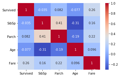
由上图可知,sibsp 和 parch 的相关度挺高,在特征处理是可能用到
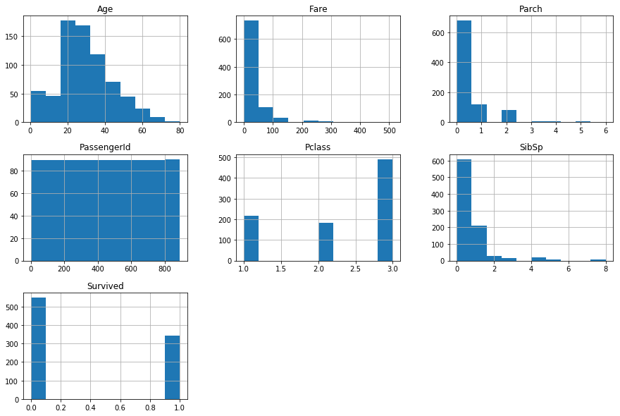
trainSet.hist(figsize=(15,10))
array([[,
        ,
        ],
       [,
        ,
        ],
       [,
        ,
        ]],
      dtype=object)
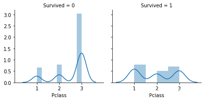
print(trainSet[["Pclass","Survived"]].groupby(["Pclass"]).mean())
g = sns.FacetGrid(trainSet,col='Survived').map(sns.distplot,'Pclass')
        Survived
Pclass
1       0.629630
2       0.472826
3       0.242363
trainSet[['Sex','Survived']].groupby(['Sex']).mean()
| Survived | |
|---|---|
| Sex | |
| female | 0.742038 |
| male | 0.188908 |
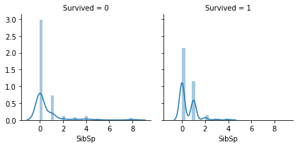
print(trainSet[['SibSp','Survived']].groupby(['SibSp']).mean())
g = sns.FacetGrid(trainSet,col='Survived').map(sns.distplot,'SibSp')
       Survived
SibSp
0      0.345395
1      0.535885
2      0.464286
3      0.250000
4      0.166667
5      0.000000
8      0.000000
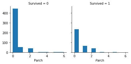
print(trainSet[['Parch','Survived']].groupby(['Parch']).mean())
g = sns.FacetGrid(trainSet, col='Survived').map(plt.hist, 'Parch')
       Survived
Parch
0      0.343658
1      0.550847
2      0.500000
3      0.600000
4      0.000000
5      0.200000
6      0.000000
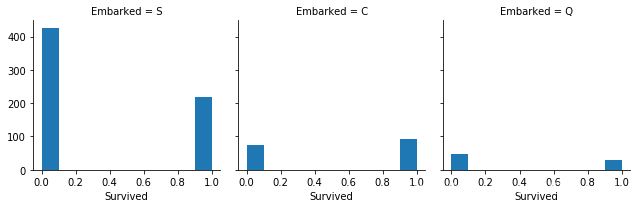
print(trainSet[['Embarked','Survived']].groupby(['Embarked']).mean())
g = sns.FacetGrid(trainSet, col='Embarked').map(plt.hist, 'Survived')
          Survived
Embarked
C         0.553571
Q         0.389610
S         0.336957
g = sns.FacetGrid(trainSet,col='Survived').map(sns.distplot,'Age')
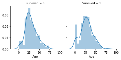
由以上存活率可以看出,这些特征对最后结果的预测还是有点影响的,婴儿和青年存活率最高
数据缺失值处理print(trainSet.isna().sum())
print('-'*50)
print(testSet.isna().sum())
PassengerId 0
Survived 0
Pclass 0
Name 0
Sex 0
Age 177
SibSp 0
Parch 0
Ticket 0
Fare 0
Cabin 687
Embarked 2
dtype: int64
--------------------------------------------------
PassengerId 0
Pclass 0
Name 0
Sex 0
Age 86
SibSp 0
Parch 0
Ticket 0
Fare 1
Cabin 327
Embarked 0
dtype: int64
由上可知,Age,Embarked,Fare是比较重要的特征,可以填补.
Cabin缺失较多,直接丢弃不使用
#对于测试数据中Fare的缺失值用所在等级的均值填补
testSet.groupby('Pclass').Fare.mean()
Pclass
1 94.280297
2 22.202104
3 12.459678
Name: Fare, dtype: float64
#找到Fare缺失的一行数据
testSet[testSet.Fare.isnull().values==True]
| PassengerId | Pclass | Name | Sex | Age | SibSp | Parch | Ticket | Fare | Cabin | Embarked | |
|---|---|---|---|---|---|---|---|---|---|---|---|
| 152 | 1044 | 3 | Storey, Mr. Thomas | male | 60.5 | 0 | 0 | 3701 | NaN | NaN | S |
#由上图可知,Pclass = 3,故用12.459678填补
testSet.Fare.fillna(12.459678,inplace=True)
testSet.Fare[152]
12.459678
#对Embarked特征用众数填补
print(trainSet.Embarked.mode())
trainSet.Embarked.fillna('S',inplace=True)
trainSet.Embarked.isnull().sum()
0 S
dtype: object
0
print(trainSet.isna().sum())
print('-'*50)
print(testSet.isna().sum())
PassengerId      0
Survived         0
Pclass           0
Name             0
Sex              0
Age            177
SibSp            0
Parch            0
Ticket           0
Fare             0
Cabin          687
Embarked         0
dtype: int64
--------------------------------------------------
PassengerId      0
Pclass           0
Name             0
Sex              0
Age             86
SibSp            0
Parch            0
Ticket           0
Fare             0
Cabin          327
Embarked         0
dtype: int64
下面对Age特征进行缺失值填补,根据Mr,Miss,Mrs,Masters 等称呼可以划分不同的年龄段,根据各个称呼的年龄均值进行填补。
trainSet['Title'] = trainSet.Name.str.extract(' ([A-Za-z]+)\.', expand=False)
pd.crosstab(trainSet['Title'],trainSet['Sex'])
trainSet = trainSet.drop('Name',axis=1)
trainSet.head()
| PassengerId | Survived | Pclass | Sex | Age | SibSp | Parch | Ticket | Fare | Cabin | Embarked | Title | |
|---|---|---|---|---|---|---|---|---|---|---|---|---|
| 0 | 1 | 0 | 3 | male | 22.0 | 1 | 0 | A/5 21171 | 7.2500 | NaN | S | Mr |
| 1 | 2 | 1 | 1 | female | 38.0 | 1 | 0 | PC 17599 | 71.2833 | C85 | C | Mrs |
| 2 | 3 | 1 | 3 | female | 26.0 | 0 | 0 | STON/O2. 3101282 | 7.9250 | NaN | S | Miss |
| 3 | 4 | 1 | 1 | female | 35.0 | 1 | 0 | 113803 | 53.1000 | C123 | S | Mrs |
| 4 | 5 | 0 | 3 | male | 35.0 | 0 | 0 | 373450 | 8.0500 | NaN | S | Mr |
trainSet.Title.value_counts()
Mr          517
Miss        182
Mrs         125
Master       40
Dr            7
Rev           6
Major         2
Mlle          2
Col           2
Ms            1
Lady          1
Don           1
Capt          1
Mme           1
Sir           1
Jonkheer      1
Countess      1
Name: Title, dtype: int64
import numpy as np
trainSet['Title'] = np.where((trainSet.Title=='Capt') | (trainSet.Title=='Countess') | (trainSet.Title=='Don') | (trainSet.Title=='Dona')
                        | (trainSet.Title=='Jonkheer')  | (trainSet.Title=='Sir') | (trainSet.Title=='Major')
                        | (trainSet.Title=='Rev') | (trainSet.Title=='Col'),'Other',trainSet.Title)
trainSet['Title'] = trainSet['Title'].replace('Ms','Miss')
trainSet['Title'] = trainSet['Title'].replace('Mlle','Miss')
trainSet['Title'] = trainSet['Title'].replace('Mme','Mrs')
trainSet['Title'] = trainSet['Title'].replace('Lady','Miss')
trainSet.Title.value_counts()
Mr        517
Miss      186
Mrs       126
Master     40
Other      15
Dr          7
Name: Title, dtype: int64
#看下不同称呼的年龄分布
sns.boxplot(data=trainSet,x='Title',y='Age')
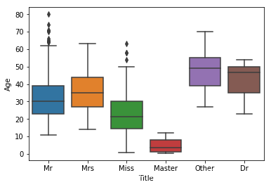
#计算不同称呼均值
trainSet.groupby('Title').Age.mean()
Title
Dr        42.000000
Master     4.574167
Miss      22.020000
Mr        32.368090
Mrs       35.788991
Other     46.800000
Name: Age, dtype: float64
#用均值进行填补
trainSet['Age'] = np.where((trainSet.Age.isnull()) & (trainSet.Title=='Master'),5,
                        np.where((trainSet.Age.isnull()) & (trainSet.Title=='Miss'),22,
                                 np.where((trainSet.Age.isnull()) & (trainSet.Title=='Mr'),32,
                                          np.where((trainSet.Age.isnull()) & (trainSet.Title=='Mrs'),36,
                                                  np.where((trainSet.Age.isnull()) & (trainSet.Title=='Other'),47,
                                                           np.where((trainSet.Age.isnull()) & (trainSet.Title=='Dr'),42,trainSet.Age))))))
trainSet.Age.isnull().sum()
0
对测试数据进行填补
testSet['Title'] = testSet.Name.str.extract(' ([A-Za-z]+)\.', expand=False)
pd.crosstab(testSet['Title'],testSet['Sex'])
testSet = testSet.drop('Name',axis=1)
testSet.Title.value_counts()
Mr        240
Miss       78
Mrs        72
Master     21
Rev         2
Col         2
Dona        1
Ms          1
Dr          1
Name: Title, dtype: int64
testSet["Title"] = np.where(((testSet["Title"]=='Rev') | (testSet["Title"]=='Col')
                                    | (testSet["Title"]=='Dona')),'Others',testSet["Title"])
testSet["Title"] = testSet["Title"].replace('Ms','Miss')
testSet.Title.value_counts()
Mr        240
Miss       79
Mrs        72
Master     21
Others      5
Dr          1
Name: Title, dtype: int64
testSet.groupby('Title').Age.mean()
Title
Dr        53.000000
Master     7.406471
Miss      21.774844
Mr        32.000000
Mrs       38.903226
Others    42.000000
Name: Age, dtype: float64
#用均值进行填补
testSet['Age'] = np.where((testSet.Age.isnull()) & (testSet.Title=='Master'),7,
                        np.where((testSet.Age.isnull()) & (testSet.Title=='Miss'),22,
                                 np.where((testSet.Age.isnull()) & (testSet.Title=='Mr'),32,
                                          np.where((testSet.Age.isnull()) & (testSet.Title=='Mrs'),39,
                                                  np.where((testSet.Age.isnull()) & (testSet.Title=='Other'),42,
                                                           np.where((testSet.Age.isnull()) & (testSet.Title=='Dr'),53,testSet.Age))))))
testSet.Age.isnull().sum()
0
#缺失值处理完成
trainSet = trainSet.drop('Cabin',axis=1)
testSet = testSet.drop('Cabin',axis=1)
print(trainSet.isnull().sum())
print('*'*50)
print(testSet.isnull().sum())
PassengerId    0
Survived       0
Pclass         0
Sex            0
Age            0
SibSp          0
Parch          0
Ticket         0
Fare           0
Embarked       0
Title          0
dtype: int64
**************************************************
PassengerId    0
Pclass         0
Sex            0
Age            0
SibSp          0
Parch          0
Ticket         0
Fare           0
Embarked       0
Title          0
dtype: int64
特征处理
新建特征:家庭总成员:Family,是否是母亲:Mother,是否免费上船:Free
trainSet['Family'] = trainSet.SibSp + trainSet.Parch + 1
trainSet['Mother'] = np.where((trainSet.Title=='Mrs') & (trainSet.Parch > 0),1,0)
trainSet['Free'] = np.where(trainSet.Fare==0,1,0)
trainSet = trainSet.drop(['SibSp','Parch'],axis=1)
trainSet.head()
| PassengerId | Survived | Pclass | Sex | Age | Ticket | Fare | Embarked | Title | Family | Mother | Free | |
|---|---|---|---|---|---|---|---|---|---|---|---|---|
| 0 | 1 | 0 | 3 | male | 22.0 | A/5 21171 | 7.2500 | S | Mr | 2 | 0 | 0 |
| 1 | 2 | 1 | 1 | female | 38.0 | PC 17599 | 71.2833 | C | Mrs | 2 | 0 | 0 |
| 2 | 3 | 1 | 3 | female | 26.0 | STON/O2. 3101282 | 7.9250 | S | Miss | 1 | 0 | 0 |
| 3 | 4 | 1 | 1 | female | 35.0 | 113803 | 53.1000 | S | Mrs | 2 | 0 | 0 |
| 4 | 5 | 0 | 3 | male | 35.0 | 373450 | 8.0500 | S | Mr | 1 | 0 | 0 |
trainSet = trainSet.drop('Ticket',axis=1)
trainSet.head()
| PassengerId | Survived | Pclass | Sex | Age | Fare | Embarked | Title | Family | Mother | Free | |
|---|---|---|---|---|---|---|---|---|---|---|---|
| 0 | 1 | 0 | 3 | male | 22.0 | 7.2500 | S | Mr | 2 | 0 | 0 |
| 1 | 2 | 1 | 1 | female | 38.0 | 71.2833 | C | Mrs | 2 | 0 | 0 |
| 2 | 3 | 1 | 3 | female | 26.0 | 7.9250 | S | Miss | 1 | 0 | 0 |
| 3 | 4 | 1 | 1 | female | 35.0 | 53.1000 | S | Mrs | 2 | 0 | 0 |
| 4 | 5 | 0 | 3 | male | 35.0 | 8.0500 | S | Mr | 1 | 0 | 0 |
testSet['Family'] = testSet.SibSp + testSet.Parch + 1
testSet['Mother'] = np.where((testSet.Title=='Mrs') & (testSet.Parch > 0),1,0)
testSet['Free'] = np.where(testSet.Fare==0,1,0)
testSet = testSet.drop(['SibSp','Parch','Ticket'],axis=1)
testSet.head()
| PassengerId | Pclass | Sex | Age | Fare | Embarked | Title | Family | Mother | Free | |
|---|---|---|---|---|---|---|---|---|---|---|
| 0 | 892 | 3 | male | 34.5 | 7.8292 | Q | Mr | 1 | 0 | 0 |
| 1 | 893 | 3 | female | 47.0 | 7.0000 | S | Mrs | 2 | 0 | 0 |
| 2 | 894 | 2 | male | 62.0 | 9.6875 | Q | Mr | 1 | 0 | 0 |
| 3 | 895 | 3 | male | 27.0 | 8.6625 | S | Mr | 1 | 0 | 0 |
| 4 | 896 | 3 | female | 22.0 | 12.2875 | S | Mrs | 3 | 1 | 0 |
#保存一下数据,防止丢失
trainSet.to_csv('work/trainSet.csv',index=0)
testSet.to_csv('work/testSet.csv',index=0)
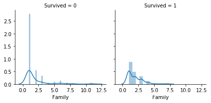
print(trainSet.groupby('Family').Survived.mean())
g = sns.FacetGrid(trainSet,col='Survived').map(sns.distplot,'Family')
Family
1     0.303538
2     0.552795
3     0.578431
4     0.724138
5     0.200000
6     0.136364
7     0.333333
8     0.000000
11    0.000000
Name: Survived, dtype: float64
trainSet.groupby('Mother').Survived.mean()
Mother
0    0.361677
1    0.714286
Name: Survived, dtype: float64
trainSet.groupby('Free').Survived.mean()
Free
0    0.389269
1    0.066667
Name: Survived, dtype: float64
#数值化处理
trainSet.head()
| PassengerId | Survived | Pclass | Sex | Age | Fare | Embarked | Title | Family | Mother | Free | |
|---|---|---|---|---|---|---|---|---|---|---|---|
| 0 | 1 | 0 | 3 | male | 22.0 | 7.2500 | S | Mr | 2 | 0 | 0 |
| 1 | 2 | 1 | 1 | female | 38.0 | 71.2833 | C | Mrs | 2 | 0 | 0 |
| 2 | 3 | 1 | 3 | female | 26.0 | 7.9250 | S | Miss | 1 | 0 | 0 |
| 3 | 4 | 1 | 1 | female | 35.0 | 53.1000 | S | Mrs | 2 | 0 | 0 |
| 4 | 5 | 0 | 3 | male | 35.0 | 8.0500 | S | Mr | 1 | 0 | 0 |
Dr 53.000000
Master 7.406471
Miss 21.774844
Mr 32.000000
Mrs 38.903226
Others
trainSet.Embarked = trainSet.Embarked.replace(['S','Q','C'],[1,2,3])
trainSet.Sex = trainSet.Sex.replace(['male','female'],[1,2])
trainSet.Title = trainSet.Title.replace(['Dr','Master','Miss','Mr','Mrs','Others'],[1,2,3,4,5,6])
trainSet.head()
| PassengerId | Survived | Pclass | Sex | Age | Fare | Embarked | Title | Family | Mother | Free | |
|---|---|---|---|---|---|---|---|---|---|---|---|
| 0 | 1 | 0 | 3 | 1 | 22.0 | 7.2500 | 1 | 4 | 2 | 0 | 0 |
| 1 | 2 | 1 | 1 | 2 | 38.0 | 71.2833 | 3 | 5 | 2 | 0 | 0 |
| 2 | 3 | 1 | 3 | 2 | 26.0 | 7.9250 | 1 | 3 | 1 | 0 | 0 |
| 3 | 4 | 1 | 1 | 2 | 35.0 | 53.1000 | 1 | 5 | 2 | 0 | 0 |
| 4 | 5 | 0 | 3 | 1 | 35.0 | 8.0500 | 1 | 4 | 1 | 0 | 0 |
testSet.Embarked = testSet.Embarked.replace(['S','Q','C'],[1,2,3])
testSet.Sex = testSet.Sex.replace(['male','female'],[1,2])
testSet.Title = testSet.Title.replace(['Dr','Master','Miss','Mr','Mrs','Others'],[1,2,3,4,5,6])
testSet.head()
| PassengerId | Pclass | Sex | Age | Fare | Embarked | Title | Family | Mother | Free | |
|---|---|---|---|---|---|---|---|---|---|---|
| 0 | 892 | 3 | 1 | 34.5 | 7.8292 | 2 | 4 | 1 | 0 | 0 |
| 1 | 893 | 3 | 2 | 47.0 | 7.0000 | 1 | 5 | 2 | 0 | 0 |
| 2 | 894 | 2 | 1 | 62.0 | 9.6875 | 2 | 4 | 1 | 0 | 0 |
| 3 | 895 | 3 | 1 | 27.0 | 8.6625 | 1 | 4 | 1 | 0 | 0 |
| 4 | 896 | 3 | 2 | 22.0 | 12.2875 | 1 | 5 | 3 | 1 | 0 |
trainSet.Age = trainSet.Age.replace(['Child', 'Young Adult', 'Adult','Older Adult','Senior'],[1,2,3,4,5])
trainSet.head()
| PassengerId | Survived | Pclass | Sex | Age | Fare | Embarked | Title | Family | Mother | Free | |
|---|---|---|---|---|---|---|---|---|---|---|---|
| 0 | 1 | 0 | 3 | 1 | 2 | 7.2500 | 1 | 4 | 2 | 0 | 0 |
| 1 | 2 | 1 | 1 | 2 | 3 | 71.2833 | 3 | 5 | 2 | 0 | 0 |
| 2 | 3 | 1 | 3 | 2 | 3 | 7.9250 | 1 | 3 | 1 | 0 | 0 |
| 3 | 4 | 1 | 1 | 2 | 3 | 53.1000 | 1 | 5 | 2 | 0 | 0 |
| 4 | 5 | 0 | 3 | 1 | 3 | 8.0500 | 1 | 4 | 1 | 0 | 0 |
bins = [0,12,24,45,60,testSet.Age.max()]
labels = [1,2,3,4,5]
testSet["Age"] = pd.cut(testSet["Age"], bins, labels = labels)
testSet.head()
| PassengerId | Pclass | Sex | Age | Fare | Embarked | Title | Family | Mother | Free | |
|---|---|---|---|---|---|---|---|---|---|---|
| 0 | 892 | 3 | 1 | 3 | 7.8292 | 2 | 4 | 1 | 0 | 0 |
| 1 | 893 | 3 | 2 | 4 | 7.0000 | 1 | 5 | 2 | 0 | 0 |
| 2 | 894 | 2 | 1 | 5 | 9.6875 | 2 | 4 | 1 | 0 | 0 |
| 3 | 895 | 3 | 1 | 3 | 8.6625 | 1 | 4 | 1 | 0 | 0 |
| 4 | 896 | 3 | 2 | 2 | 12.2875 | 1 | 5 | 3 | 1 | 0 |
#保存一下数据,防止丢失
trainSet.to_csv('work/trainSet1.csv',index=0)
/tbody>
作者:QianLong_
相关文章
Angie
2020-11-03
Jacinda
2020-06-30
Winema
2020-09-03
Kita
2021-05-30
Rachel
2023-07-20
Psyche
2023-07-20
Winola
2023-07-20
Gella
2023-07-20
Grizelda
2023-07-20
Janna
2023-07-20
Ophelia
2023-07-21
Crystal
2023-07-21
Laila
2023-07-21
Aine
2023-07-21
Bliss
2023-07-21
Lillian
2023-07-21
Tertia
2023-07-21
Olive
2023-07-21