吴恩达深度学习第一课--第四周多层神经网络实现
本文参考何宽、念师
前言本次教程,将构建两个神经网络,一个是具有两个隐藏层的神经网络,一个是多隐藏层的神经网络。
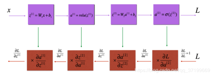
一个神经网络的计算过程如下:
import numpy as np
import h5py
import matplotlib.pyplot as plt
import testCases #参见资料包,或者在文章底部copy
from dnn_utils import sigmoid, sigmoid_backward, relu, relu_backward #参见资料包
import lr_utils #参见资料包,或者在文章底部copy
np.random.seed(1)
其中,sigmoid函数如下:
def sigmoid(Z):
    """
    Implements the sigmoid activation in numpy
    Arguments:
    Z -- numpy array of any shape
    Returns:
    A -- output of sigmoid(z), same shape as Z
    cache -- returns Z as well, useful during backpropagation
    """
    A = 1/(1+np.exp(-Z))
    cache = Z
    return A, cache
sigmoid_backward函数如下:
def sigmoid_backward(dA, cache):
    """
    Implement the backward propagation for a single SIGMOID unit.
    Arguments:
    dA -- post-activation gradient, of any shape
    cache -- 'Z' where we store for computing backward propagation efficiently
    Returns:
    dZ -- Gradient of the cost with respect to Z
    """
    Z = cache
    s = 1/(1+np.exp(-Z))
    dZ = dA * s * (1-s)
    assert (dZ.shape == Z.shape)
    return dZ
relu函数如下:
def relu(Z):
    """
    Implement the RELU function.
    Arguments:
    Z -- Output of the linear layer, of any shape
    Returns:
    A -- Post-activation parameter, of the same shape as Z
    cache -- a python dictionary containing "A" ; stored for computing the backward pass efficiently
    """
    A = np.maximum(0,Z)
    assert(A.shape == Z.shape)
    cache = Z
    return A, cache
relu_backward函数如下:
def relu_backward(dA, cache):
    """
    Implement the backward propagation for a single RELU unit.
    Arguments:
    dA -- post-activation gradient, of any shape
    cache -- 'Z' where we store for computing backward propagation efficiently
    Returns:
    dZ -- Gradient of the cost with respect to Z
    """
    Z = cache
    dZ = np.array(dA, copy=True) # just converting dz to a correct object.
    # When z <= 0, you should set dz to 0 as well.
    dZ[Z <= 0] = 0
    assert (dZ.shape == Z.shape)
    return dZ
初始化参数
对于一个两层的神经网络而言,模型结构是:线性–>Relu–>线性–>sigmoid函数。
初始化函数如下:
def initialize_parameters(n_x,n_h,n_y):
    """
    此函数是为了初始化两层网络参数而使用的函数。
    参数:
        n_x - 输入层节点数量
        n_h - 隐藏层节点数量
        n_y - 输出层节点数量
    返回:
        parameters - 包含你的参数的python字典:
            W1 - 权重矩阵,维度为(n_h,n_x)
            b1 - 偏向量,维度为(n_h,1)
            W2 - 权重矩阵,维度为(n_y,n_h)
            b2 - 偏向量,维度为(n_y,1)
    """
    W1 = np.random.randn(n_h, n_x) * 0.01
    b1 = np.zeros((n_h, 1))
    W2 = np.random.randn(n_y, n_h) * 0.01
    b2 = np.zeros((n_y, 1))
    #使用断言确保我的数据格式是正确的
    assert(W1.shape == (n_h, n_x))
    assert(b1.shape == (n_h, 1))
    assert(W2.shape == (n_y, n_h))
    assert(b2.shape == (n_y, 1))
    parameters = {"W1": W1,
                  "b1": b1,
                  "W2": W2,
                  "b2": b2}
    return parameters
测试:
parameters = initialize_parameters(3,2,1)
print("W1 = " + str(parameters["W1"]))
print("b1 = " + str(parameters["b1"]))
print("W2 = " + str(parameters["W2"]))
print("b2 = " + str(parameters["b2"]))
结果:
W1 = [[ 0.01624345 -0.00611756 -0.00528172]
 [-0.01072969  0.00865408 -0.02301539]]
b1 = [[0.]
 [0.]]
W2 = [[ 0.01744812 -0.00761207]]
b2 = [[0.]]
两层神经网络测试完毕,那么对于一个L层的神经网络而言呢?初始化会是什么样的?
其中,W[l]W^{[l]}W[l]维度为(layers_dims [l],layers_dims [l-1]),b[l]b^{[l]}b[l]维度为(layers_dims [l],1)。
def initialize_parameters_deep(layers_dims):
    """
    此函数是为了初始化多层网络参数而使用的函数。
    参数:
        layers_dims - 包含我们网络中每个图层的节点数量的列表
    返回:
        parameters - 包含参数“W1”,“b1”,...,“WL”,“bL”的字典:
                     W1 - 权重矩阵,维度为(layers_dims [1],layers_dims [1-1])
                     bl - 偏向量,维度为(layers_dims [1],1)
    """
    np.random.seed(3)
    parameters = {}
    L = len(layers_dims)
    for l in range(1,L):
        parameters['W'+str(l)] = np.random.randn(layers_dims[l],layers_dims[l-1]) / np.sqrt(layers_dims[l-1])
        parameters['b'+str(l)] = np.zeros((layers_dims[l],1))
        #确保我要的数据的格式是正确的
        assert(parameters["W" + str(l)].shape == (layers_dims[l], layers_dims[l-1]))
        assert(parameters["b" + str(l)].shape == (layers_dims[l], 1))
    return parameters
测试:
layers_dims = [5,4,3]
parameters = initialize_parameters_deep(layers_dims)
print("W1 = " + str(parameters["W1"]))
print("b1 = " + str(parameters["b1"]))
print("W2 = " + str(parameters["W2"]))
print("b2 = " + str(parameters["b2"]))
结果:
W1 = [[ 0.79989897  0.19521314  0.04315498 -0.83337927 -0.12405178]
 [-0.15865304 -0.03700312 -0.28040323 -0.01959608 -0.21341839]
 [-0.58757818  0.39561516  0.39413741  0.76454432  0.02237573]
 [-0.18097724 -0.24389238 -0.69160568  0.43932807 -0.49241241]]
b1 = [[0.]
 [0.]
 [0.]
 [0.]]
W2 = [[-0.59252326 -0.10282495  0.74307418  0.11835813]
 [-0.51189257 -0.3564966   0.31262248 -0.08025668]
 [-0.38441818 -0.11501536  0.37252813  0.98805539]]
b2 = [[0.]
 [0.]
 [0.]]
自此,我们已经分别构建了两层和多层神经网络的初始化参数的函数,现在开始构建前向传播函数。
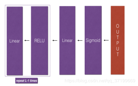
前向传播函数前向传播有以下三个步骤:
linear linear–>avtivation,其中激活函数使用Relu或sigmoid。 [linear–>Relu]x(L-1)–>linear–>sigmoid(整个模型)。其中,
Z[L]=W[L]A[L−1]+b[L]Z^{[L]}=W^{[L]}A^{[L-1]}+b^{[L]}Z[L]=W[L]A[L−1]+b[L]
A[L]=g[L](Z[L])=g[L](W[L]A[L−1]+b[L])A^{[L]}=g^{[L]}(Z^{[L]})=g^{[L]}(W^{[L]}A^{[L-1]}+b^{[L]})A[L]=g[L](Z[L])=g[L](W[L]A[L−1]+b[L])
def linear_forward(A,W,b):
    """
    实现前向传播的线性部分。
    参数:
        A - 来自上一层(或输入数据)的激活,维度为(上一层的节点数量,示例的数量)
        W - 权重矩阵,numpy数组,维度为(当前图层的节点数量,前一图层的节点数量)
        b - 偏向量,numpy向量,维度为(当前图层节点数量,1)
    返回:
         Z - 激活功能的输入,也称为预激活参数
         cache - 一个包含“A”,“W”和“b”的字典,存储这些变量以有效地计算后向传递
    """
    Z = np.dot(W,A) + b
    assert(Z.shape == (W.shape[0],A.shape[1]))
    cache = (A,W,b)
    return Z,cache
测试
print("==============测试linear_forward==============")
A,W,b = testCases.linear_forward_test_case()
Z,linear_cache = linear_forward(A,W,b)
print("Z = " + str(Z))
结果:
Z = [[ 3.26295337 -1.23429987]]
线性激活部分linear–>avtivation
def linear_activation_forward(A_prev,W,b,activation):
    """
    实现LINEAR-> ACTIVATION 这一层的前向传播
    参数:
        A_prev - 来自上一层(或输入层)的激活,维度为(上一层的节点数量,示例数)
        W - 权重矩阵,numpy数组,维度为(当前层的节点数量,前一层的大小)
        b - 偏向量,numpy阵列,维度为(当前层的节点数量,1)
        activation - 选择在此层中使用的激活函数名,字符串类型,【"sigmoid" | "relu"】
    返回:
        A - 激活函数的输出,也称为激活后的值
        cache - 一个包含“linear_cache”和“activation_cache”的字典,我们需要存储它以有效地计算后向传递
    """
    if activation == "sigmoid":
        Z, linear_cache = linear_forward(A_prev, W, b)
        A, activation_cache = sigmoid(Z)
    elif activation == "relu":
        Z, linear_cache = linear_forward(A_prev, W, b)
        A, activation_cache = relu(Z)
    assert(A.shape == (W.shape[0],A_prev.shape[1]))
    cache = (linear_cache,activation_cache)
    return A,cache
测试:
A_prev, W,b = testCases.linear_activation_forward_test_case()
A, linear_activation_cache = linear_activation_forward(A_prev, W, b, activation = "sigmoid")
print("sigmoid,A = " + str(A))
A, linear_activation_cache = linear_activation_forward(A_prev, W, b, activation = "relu")
print("ReLU,A = " + str(A))
结果:
sigmoid,A = [[0.96890023 0.11013289]]
ReLU,A = [[3.43896131 0.        ]]
多层模型的前向传播计算模型代码如下:
def L_model_forward(X,parameters):
    """
    实现[LINEAR-> RELU] *(L-1) - > LINEAR-> SIGMOID计算前向传播,也就是多层网络的前向传播,为后面每一层都执行LINEAR和ACTIVATION
    参数:
        X - 数据,numpy数组,维度为(输入节点数量,示例数)
        parameters - initialize_parameters_deep()的输出
    返回:
        AL - 最后的激活值
        caches - 包含以下内容的缓存列表:
                 linear_relu_forward()的每个cache(有L-1个,索引为从0到L-2)
                 linear_sigmoid_forward()的cache(只有一个,索引为L-1)
    """
    caches = []
    A = X
    L = len(parameters) // 2
    for l in range(1,L):
        A_prev = A
        A, cache = linear_activation_forward(A_prev, parameters['W' + str(l)], parameters['b' + str(l)], "relu")
        caches.append(cache)
    AL, cache = linear_activation_forward(A, parameters['W' + str(L)], parameters['b' + str(L)], "sigmoid")
    caches.append(cache)
    assert(AL.shape == (1,X.shape[1]))
    return AL,caches
测试:
X,parameters = testCases.L_model_forward_test_case()
AL,caches = L_model_forward(X,parameters)
print("AL = " + str(AL))
print("caches 的长度为 = " + str(len(caches)))
结果:
AL = [[0.17007265 0.2524272 ]]
caches 的长度为 = 2
计算成本
def compute_cost(AL,Y):
    """
    实施等式(4)定义的成本函数。
    参数:
        AL - 与标签预测相对应的概率向量,维度为(1,示例数量)
        Y - 标签向量(例如:如果不是猫,则为0,如果是猫则为1),维度为(1,数量)
    返回:
        cost - 交叉熵成本
    """
    m = Y.shape[1]
    cost = -np.sum(np.multiply(np.log(AL),Y) + np.multiply(np.log(1 - AL), 1 - Y)) / m
    cost = np.squeeze(cost)
    assert(cost.shape == ())
    return cost
测试:
Y,AL = testCases.compute_cost_test_case()
print("cost = " + str(compute_cost(AL, Y)))
结果:
cost = 0.414931599615397
反向传播
反向传播用于计算相对于参数的损失函数的梯度,来看看向前、向后传播的流程图:
对于线性部分,反向传播的公式如下:
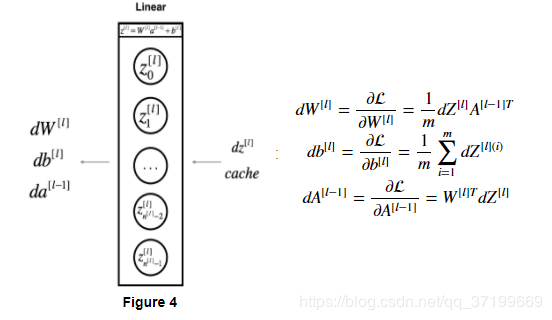
与前向传播类似,使用三个步骤来构建反向传播:
def linear_backward(dZ,cache):
    """
    为单层实现反向传播的线性部分(第L层)
    参数:
         dZ - 相对于(当前第l层的)线性输出的成本梯度
         cache - 来自当前层前向传播的值的元组(A_prev,W,b)
    返回:
         dA_prev - 相对于激活(前一层l-1)的成本梯度,与A_prev维度相同
         dW - 相对于W(当前层l)的成本梯度,与W的维度相同
         db - 相对于b(当前层l)的成本梯度,与b维度相同
    """
    A_prev, W, b = cache
    m = A_prev.shape[1]
    dW = np.dot(dZ, A_prev.T) / m
    db = np.sum(dZ, axis=1, keepdims=True) / m
    dA_prev = np.dot(W.T, dZ)
    assert (dA_prev.shape == A_prev.shape)
    assert (dW.shape == W.shape)
    assert (db.shape == b.shape)
    return dA_prev, dW, db
测试:
dZ, linear_cache = testCases.linear_backward_test_case()
dA_prev, dW, db = linear_backward(dZ, linear_cache)
print ("dA_prev = "+ str(dA_prev))
print ("dW = " + str(dW))
print ("db = " + str(db))
结果:
dA_prev = [[ 0.51822968 -0.19517421]
 [-0.40506361  0.15255393]
 [ 2.37496825 -0.89445391]]
dW = [[-0.10076895  1.40685096  1.64992505]]
db = [[0.50629448]]
线性激活部分linear–>activation backward
def linear_activation_backward(dA,cache,activation="relu"):
    """
    实现LINEAR-> ACTIVATION层的后向传播。
    参数:
         dA - 当前层l的激活后的梯度值
         cache - 我们存储的用于有效计算反向传播的值的元组(值为linear_cache,activation_cache)
         activation - 要在此层中使用的激活函数名,字符串类型,【"sigmoid" | "relu"】
    返回:
         dA_prev - 相对于激活(前一层l-1)的成本梯度值,与A_prev维度相同
         dW - 相对于W(当前层l)的成本梯度值,与W的维度相同
         db - 相对于b(当前层l)的成本梯度值,与b的维度相同
    """
    linear_cache, activation_cache = cache
    if activation == "relu":
        dZ = relu_backward(dA, activation_cache)
        dA_prev, dW, db = linear_backward(dZ, linear_cache)
    elif activation == "sigmoid":
        dZ = sigmoid_backward(dA, activation_cache)
        dA_prev, dW, db = linear_backward(dZ, linear_cache)
    return dA_prev,dW,db
测试:
AL, linear_activation_cache = testCases.linear_activation_backward_test_case()
dA_prev, dW, db = linear_activation_backward(AL, linear_activation_cache, activation = "sigmoid")
print ("sigmoid:")
print ("dA_prev = "+ str(dA_prev))
print ("dW = " + str(dW))
print ("db = " + str(db) + "\n")
dA_prev, dW, db = linear_activation_backward(AL, linear_activation_cache, activation = "relu")
print ("relu:")
print ("dA_prev = "+ str(dA_prev))
print ("dW = " + str(dW))
print ("db = " + str(db))
结果:
sigmoid:
dA_prev = [[ 0.11017994  0.01105339]
 [ 0.09466817  0.00949723]
 [-0.05743092 -0.00576154]]
dW = [[ 0.10266786  0.09778551 -0.01968084]]
db = [[-0.05729622]]
relu:
dA_prev = [[ 0.44090989 -0.        ]
 [ 0.37883606 -0.        ]
 [-0.2298228   0.        ]]
dW = [[ 0.44513824  0.37371418 -0.10478989]]
db = [[-0.20837892]]
对于L层神经网络,其反向传播函数如下:
def L_model_backward(AL,Y,caches):
    """
    对[LINEAR-> RELU] *(L-1) - > LINEAR - > SIGMOID组执行反向传播,就是多层网络的向后传播
    参数:
     AL - 概率向量,正向传播的输出(L_model_forward())
     Y - 标签向量(例如:如果不是猫,则为0,如果是猫则为1),维度为(1,数量)
     caches - 包含以下内容的cache列表:
                 linear_activation_forward("relu")的cache,不包含输出层
                 linear_activation_forward("sigmoid")的cache
    返回:
     grads - 具有梯度值的字典
              grads [“dA”+ str(l)] = ...
              grads [“dW”+ str(l)] = ...
              grads [“db”+ str(l)] = ...
    """
    grads = {}
    L = len(caches)
    m = AL.shape[1]
    Y = Y.reshape(AL.shape)
    dAL = - (np.divide(Y, AL) - np.divide(1 - Y, 1 - AL))
    current_cache = caches[L-1]
    grads["dA" + str(L)], grads["dW" + str(L)], grads["db" + str(L)] = linear_activation_backward(dAL, current_cache, "sigmoid")
    for l in reversed(range(L-1)):
        current_cache = caches[l]
        dA_prev_temp, dW_temp, db_temp = linear_activation_backward(grads["dA" + str(l + 2)], current_cache, "relu")
        grads["dA" + str(l + 1)] = dA_prev_temp
        grads["dW" + str(l + 1)] = dW_temp
        grads["db" + str(l + 1)] = db_temp
    return grads
测试:
AL, Y_assess, caches = testCases.L_model_backward_test_case()
grads = L_model_backward(AL, Y_assess, caches)
print ("dW1 = "+ str(grads["dW1"]))
print ("db1 = "+ str(grads["db1"]))
print ("dA1 = "+ str(grads["dA1"]))
结果:
dW1 = [[0.41010002 0.07807203 0.13798444 0.10502167]
 [0.         0.         0.         0.        ]
 [0.05283652 0.01005865 0.01777766 0.0135308 ]]
db1 = [[-0.22007063]
 [ 0.        ]
 [-0.02835349]]
dA1 = [[ 0.          0.52257901]
 [ 0.         -0.3269206 ]
 [ 0.         -0.32070404]
 [ 0.         -0.74079187]]
更新参数
更新参数公式如下:
W[L]=W[L]−αdW[L]W^{[L]}=W^{[L]}-\alpha dW^{[L]}W[L]=W[L]−αdW[L]
b[L]=b[L]−αdb[L]b^{[L]}=b^{[L]}-\alpha db^{[L]}b[L]=b[L]−αdb[L]
def update_parameters(parameters, grads, learning_rate):
    """
    使用梯度下降更新参数
    参数:
     parameters - 包含你的参数的字典
     grads - 包含梯度值的字典,是L_model_backward的输出
    返回:
     parameters - 包含更新参数的字典
                   参数[“W”+ str(l)] = ...
                   参数[“b”+ str(l)] = ...
    """
    L = len(parameters) // 2 #整除
    for l in range(1,L):
        parameters["W" + str(l)] = parameters["W" + str(l)] - learning_rate * grads["dW" + str(l)]
        parameters["b" + str(l)] = parameters["b" + str(l)] - learning_rate * grads["db" + str(l)]
    return parameters
测试:
parameters, grads = testCases.update_parameters_test_case()
parameters = update_parameters(parameters, grads, 0.1)
print ("W1 = "+ str(parameters["W1"]))
print ("b1 = "+ str(parameters["b1"]))
print ("W2 = "+ str(parameters["W2"]))
print ("b2 = "+ str(parameters["b2"]))
结果:
W1 = [[-0.59562069 -0.09991781 -2.14584584  1.82662008]
 [-1.76569676 -0.80627147  0.51115557 -1.18258802]
 [-1.0535704  -0.86128581  0.68284052  2.20374577]]
b1 = [[-0.04659241]
 [-1.28888275]
 [ 0.53405496]]
W2 = [[-0.55569196  0.0354055   1.32964895]]
b2 = [[-0.84610769]]
整合
至此,已经实现该神经网络中所有需要的函数,接下来,将这些方法组合在一起,构成一个神经网络类。
两层神经网络模型def two_layer_model(X,Y,layers_dims,learning_rate=0.0075,num_iterations=3000,print_cost=False,isPlot=True):
"""
实现一个两层的神经网络,【LINEAR->RELU】 -> 【LINEAR->SIGMOID】
参数:
X - 输入的数据,维度为(n_x,例子数)
Y - 标签,向量,0为非猫,1为猫,维度为(1,数量)
layers_dims - 层数的向量,维度为(n_y,n_h,n_y)
learning_rate - 学习率
num_iterations - 迭代的次数
print_cost - 是否打印成本值,每100次打印一次
isPlot - 是否绘制出误差值的图谱
返回:
parameters - 一个包含W1,b1,W2,b2的字典变量
"""
np.random.seed(1)
grads = {}
costs = []
(n_x,n_h,n_y) = layers_dims
"""
初始化参数
"""
parameters = initialize_parameters(n_x, n_h, n_y)
W1 = parameters["W1"]
b1 = parameters["b1"]
W2 = parameters["W2"]
b2 = parameters["b2"]
"""
开始进行迭代
"""
for i in range(0,num_iterations):
#前向传播
A1, cache1 = linear_activation_forward(X, W1, b1, "relu")
A2, cache2 = linear_activation_forward(A1, W2, b2, "sigmoid")
#计算成本
cost = compute_cost(A2,Y)
#后向传播
##初始化后向传播
dA2 = - (np.divide(Y, A2) - np.divide(1 - Y, 1 - A2))
##向后传播,输入:“dA2,cache2,cache1”。 输出:“dA1,dW2,db2;还有dA0(未使用),dW1,db1”。
dA1, dW2, db2 = linear_activation_backward(dA2, cache2, "sigmoid")
dA0, dW1, db1 = linear_activation_backward(dA1, cache1, "relu")
##向后传播完成后的数据保存到grads
grads["dW1"] = dW1
grads["db1"] = db1
grads["dW2"] = dW2
grads["db2"] = db2
#更新参数
parameters = update_parameters(parameters,grads,learning_rate)
W1 = parameters["W1"]
b1 = parameters["b1"]
W2 = parameters["W2"]
b2 = parameters["b2"]
#打印成本值,如果print_cost=False则忽略
if i % 100 == 0:
#记录成本
costs.append(cost)
#是否打印成本值
if print_cost:
print("第", i ,"次迭代,成本值为:" ,np.squeeze(cost))
#迭代完成,根据条件绘制图
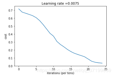
if isPlot:
plt.plot(np.squeeze(costs))
plt.ylabel('cost')
plt.xlabel('iterations (per tens)')
plt.title("Learning rate =" + str(learning_rate))
plt.show()
#返回parameters
return parameters
测试:
train_set_x_orig , train_set_y , test_set_x_orig , test_set_y , classes = lr_utils.load_dataset()
train_x_flatten = train_set_x_orig.reshape(train_set_x_orig.shape[0], -1).T
test_x_flatten = test_set_x_orig.reshape(test_set_x_orig.shape[0], -1).T
train_x = train_x_flatten / 255
train_y = train_set_y
test_x = test_x_flatten / 255
test_y = test_set_y
n_x = 12288
n_h = 7
n_y = 1
layers_dims = (n_x,n_h,n_y)
parameters = two_layer_model(train_x, train_set_y, layers_dims = (n_x, n_h, n_y), num_iterations = 1000, print_cost=True,isPlot=True)
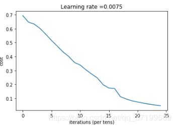
结果:
第 0 次迭代,成本值为: 0.6930497356599891
第 100 次迭代,成本值为: 0.6464320953428849
第 200 次迭代,成本值为: 0.6325140647912678
第 300 次迭代,成本值为: 0.6015024920354665
第 400 次迭代,成本值为: 0.5601966311605748
第 500 次迭代,成本值为: 0.515830477276473
第 600 次迭代,成本值为: 0.47549013139433266
第 700 次迭代,成本值为: 0.4339163151225749
第 800 次迭代,成本值为: 0.4007977536203886
第 900 次迭代,成本值为: 0.35807050113237976
预测部分:
def predict(X, y, parameters):
    """
    该函数用于预测L层神经网络的结果,当然也包含两层
    参数:
     X - 测试集
     y - 标签
     parameters - 训练模型的参数
    返回:
     p - 给定数据集X的预测
    """
    m = X.shape[1]
    n = len(parameters) // 2 # 神经网络的层数
    p = np.zeros((1,m))
    #根据参数前向传播
    probas, caches = L_model_forward(X, parameters)
    for i in range(0, probas.shape[1]):
        if probas[0,i] > 0.5:
            p[0,i] = 1
        else:
            p[0,i] = 0
    print("准确度为: "  + str(float(np.sum((p == y))/m)))
    return p
测试:
predictions_train = predict(train_x, train_y, parameters) #训练集
predictions_test = predict(test_x, test_y, parameters) #测试集
结果:
准确度为: 1.0
准确度为: 0.72
L层神经网络
def L_layer_model(X, Y, layers_dims, learning_rate=0.0075, num_iterations=3000, print_cost=False,isPlot=True):
    """
    实现一个L层神经网络:[LINEAR-> RELU] *(L-1) - > LINEAR-> SIGMOID。
    参数:
	    X - 输入的数据,维度为(n_x,例子数)
        Y - 标签,向量,0为非猫,1为猫,维度为(1,数量)
        layers_dims - 层数的向量,维度为(n_y,n_h,···,n_h,n_y)
        learning_rate - 学习率
        num_iterations - 迭代的次数
        print_cost - 是否打印成本值,每100次打印一次
        isPlot - 是否绘制出误差值的图谱
    返回:
     parameters - 模型学习的参数。 然后他们可以用来预测。
    """
    np.random.seed(1)
    costs = []
    parameters = initialize_parameters_deep(layers_dims)
    for i in range(0,num_iterations):
        AL , caches = L_model_forward(X,parameters)
        cost = compute_cost(AL,Y)
        grads = L_model_backward(AL,Y,caches)
        parameters = update_parameters(parameters,grads,learning_rate)
        #打印成本值,如果print_cost=False则忽略
        if i % 100 == 0:
            #记录成本
            costs.append(cost)
            #是否打印成本值
            if print_cost:
                print("第", i ,"次迭代,成本值为:" ,np.squeeze(cost))
    #迭代完成,根据条件绘制图
    if isPlot:
        plt.plot(np.squeeze(costs))
        plt.ylabel('cost')
        plt.xlabel('iterations (per tens)')
        plt.title("Learning rate =" + str(learning_rate))
        plt.show()
    return parameters
测试:
layers_dims = [12288, 20, 7, 5, 1] #  5-layer model
parameters = L_layer_model(train_x, train_y, layers_dims, num_iterations = 1000, print_cost = True,isPlot=True)
结果:
第 0 次迭代,成本值为: 0.715731513413713
第 100 次迭代,成本值为: 0.6747377593469114
第 200 次迭代,成本值为: 0.6603365433622127
第 300 次迭代,成本值为: 0.6462887802148751
第 400 次迭代,成本值为: 0.6298131216927773
第 500 次迭代,成本值为: 0.606005622926534
第 600 次迭代,成本值为: 0.5690041263975134
第 700 次迭代,成本值为: 0.519796535043806
第 800 次迭代,成本值为: 0.46415716786282285
第 900 次迭代,成本值为: 0.40842030048298916
预测部分测试:
train_set_x_orig , train_set_y , test_set_x_orig , test_set_y , classes = lr_utils.load_dataset()
train_x_flatten = train_set_x_orig.reshape(train_set_x_orig.shape[0], -1).T
test_x_flatten = test_set_x_orig.reshape(test_set_x_orig.shape[0], -1).T
train_x = train_x_flatten / 255
train_y = train_set_y
test_x = test_x_flatten / 255
test_y = test_set_y
pred_train = predict(train_x, train_y, parameters) #训练集
pred_test = predict(test_x, test_y, parameters) #测试集
结果:
准确度为: 0.9952153110047847
准确度为: 0.78
分析
可以看一看有哪些东西在L层模型找哪个被错误地标记了,导致准确率没有提高。
def print_mislabeled_images(classes,X,y,p):
    a = p+y
    mislabeled_indices = np.asarray(np.where(a==1))
    plt.rcParams['figure.figsize'] = (40.0,40.0)
    num_images = len(mislabeled_indices[0])
    for i in range(num_images):
        index = mislabeled_indices[1][i]
        plt.subplot(2,num_images,i+1)
        plt.imshow(X[:,index].reshape(64,64,3),interpolation='nearest')
        plt.axis('off')
        plt.title("Prediction:"+classes[int(p[0,index])].decode("utf-8")+"\n Class:"+classes[y[0,index]].decode("utf-8"))
print_mislabeled_images(classes,test_x,test_y,pred_test)
结果:
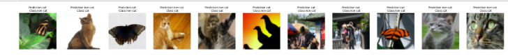
分析一下就得知原因:模型往往表现欠佳的几种类型图形包括:
测试本地电脑图片:
from skimage import transform
my_image = "tim.jpg"
my_label_y = [1]
fname = "D:/20200112zhaohuan/"+my_image
image = plt.imread(fname,'rb')
plt.imshow(image)
my_image = transform.resize(image,(64,64,3)).reshape(64*64*3,1)
my_predicted_image = predict(my_image,my_label_y,parameters)
print("y = "+str(np.squeeze(my_predicted_image))+",your L-layer model predicts a \"" + classes[int(np.squeeze(my_predicted_image)),].decode("utf-8")+"\"picture.")
结果:
(455, 640, 3)
(12288, 1)
准确度为: 0.0
y = 0.0,your L-layer model predicts a "non-cat"picture.

看来并不是所有的图片都能识别呢!
作者:zhaohuan_1996