深度学习项目之mnist手写数字识别实战(TensorFlow框架)
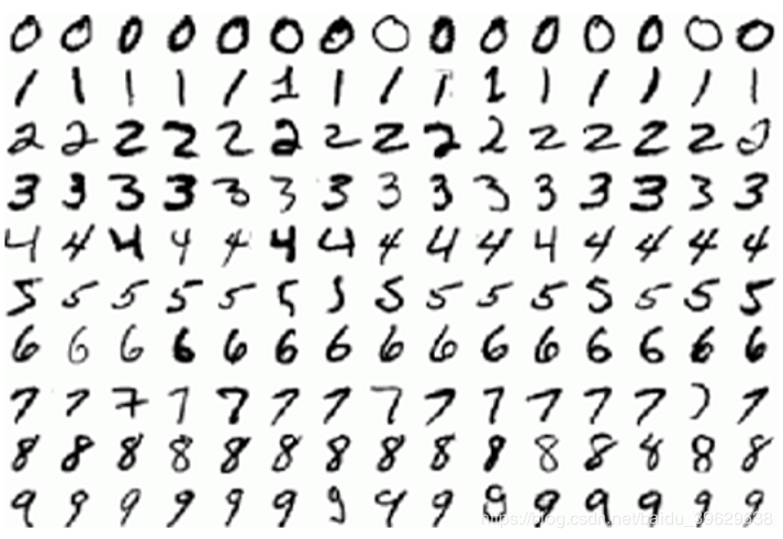
mnist手写数字识别是所有深度学习开发者的必经之路,mnist数据集的图片十分简单,是二值化图像,像素个数为28x28。所以对于所有研究深度学习的开发者来说学会mnist数据集的模型十分有必要。以此为实例进行计算机视觉如何进行识别出图片中的数据。
MNIST手写数字数据集来自美国国家标准与技术研究所,National Institute of Standards and Technology (NIST)。 训练集 (training set) 由来自 250 个不同人手写的数字构成,其中50%是高中学生,50% 来自人口普查局 (the Census Bureau) 的工作人员。测试集(test set) 也是同样比例的手写数字数据。
mnist数据集的重要参数如下:
train数据集:60000张图片数据
test数据集:10000张图片数据
图片分辨率大小:28x28
接下来就是如何构建一个神经网络的模型使得让计算机可以识别出图像中过得数字即可
docker:
win10操作系统/ubuntu系统,anaconda环境
TensorFlow·1.13.0,python3.7,pycharm2017
友情提示:很多同学在搭建深度学习环境中会遇到很多问题,尤其是安装TensorFlow框架时,TensorFlow是Google公司的深度学习框架,所以在执行pip安装时候会报错read time out 所以需要网速快还有梯子等。
下面直接进入代码
首先撰写脚本代码下载mnist数据集的input数据并且打印张量显示
download.py
# coding:utf-8
# 从tensorflow.examples.tutorials.mnist引入模块。这是TensorFlow为了教学MNIST而提前编制的程序
from tensorflow.examples.tutorials.mnist import input_data
# 从MNIST_data/中读取MNIST数据。这条语句在数据不存在时,会自动执行下载
mnist = input_data.read_data_sets("MNIST_data/", one_hot=True)
# 查看训练数据的大小
print(mnist.train.images.shape)  # (55000, 784)
print(mnist.train.labels.shape)  # (55000, 10)
# 查看验证数据的大小
print(mnist.validation.images.shape)  # (5000, 784)
print(mnist.validation.labels.shape)  # (5000, 10)
# 查看测试数据的大小
print(mnist.test.images.shape)  # (10000, 784)
print(mnist.test.labels.shape)  # (10000, 10)
# 打印出第0幅图片的向量表示
print(mnist.train.images[0, :])
# 打印出第0幅图片的标签
print(mnist.train.labels[0, :])
接下来一步其实可有可无,如mnist数据集·有一些了解的话其实可以直接跳过
save_picture.py
#coding: utf-8
from tensorflow.examples.tutorials.mnist import input_data
import scipy.misc
import os
# 读取MNIST数据集。如果不存在会事先下载。
mnist = input_data.read_data_sets("MNIST_data/", one_hot=True)
# 我们把原始图片保存在MNIST_data/raw/文件夹下
# 如果没有这个文件夹会自动创建
save_dir = 'MNIST_data/raw/'
if os.path.exists(save_dir) is False:
    os.makedirs(save_dir)
# 保存前20张图片
for i in range(20):
    # 请注意,mnist.train.images[i, :]就表示第i张图片(序号从0开始)
    image_array = mnist.train.images[i, :]
    # TensorFlow中的MNIST图片是一个784维的向量,我们重新把它还原为28x28维的图像。
    image_array = image_array.reshape(28, 28)
    # 保存文件的格式为 mnist_train_0.jpg, mnist_train_1.jpg, ... ,mnist_train_19.jpg
    filename = save_dir + 'mnist_train_%d.jpg' % i
    # 将image_array保存为图片
    # 先用scipy.misc.toimage转换为图像,再调用save直接保存。
    scipy.misc.toimage(image_array, cmin=0.0, cmax=1.0).save(filename)
print('Please check: %s ' % save_dir)
array转换为image的代码中最核心的就是scripy.misc.toimage()
最后放入save_dir文件夹
在进行完数据集的下载后进行数据集的label打印
print_label.py
#coding: utf-8
from tensorflow.examples.tutorials.mnist import input_data
import scipy.misc
import os
# 读取MNIST数据集。如果不存在会事先下载。
mnist = input_data.read_data_sets("MNIST_data/", one_hot=True)
# 我们把原始图片保存在MNIST_data/raw/文件夹下
# 如果没有这个文件夹会自动创建
save_dir = 'MNIST_data/raw/'
if os.path.exists(save_dir) is False:
    os.makedirs(save_dir)
# 保存前20张图片
for i in range(20):
    # 请注意,mnist.train.images[i, :]就表示第i张图片(序号从0开始)
    image_array = mnist.train.images[i, :]
    # TensorFlow中的MNIST图片是一个784维的向量,我们重新把它还原为28x28维的图像。
    image_array = image_array.reshape(28, 28)
    # 保存文件的格式为 mnist_train_0.jpg, mnist_train_1.jpg, ... ,mnist_train_19.jpg
    filename = save_dir + 'mnist_train_%d.jpg' % i
    # 将image_array保存为图片
    # 先用scipy.misc.toimage转换为图像,再调用save直接保存。
    scipy.misc.toimage(image_array, cmin=0.0, cmax=1.0).save(filename)
print('Please check: %s ' % save_dir)
softmax.py
采用在这份代码中是类似机器学习中的单层全连接层采用随机梯度下降的算法并且学习率为0.0001,tf.train.GradientDescentOptimizer代码是TensorFlow框架中集成的优化器0.01则是learning rate代表学习率
代码运行后发现accuracy并不是很高,really!mnist数据集随随便便就可以95%
# coding:utf-8
# 导入tensorflow。
# 这句import tensorflow as tf是导入TensorFlow约定俗成的做法,请大家记住。
import tensorflow as tf
# 导入MNIST教学的模块
import os
os.environ['TF_CPP_MIN_LOG_LEVEL']='2'
from tensorflow.examples.tutorials.mnist import input_data
# 与之前一样,读入MNIST数据
mnist = input_data.read_data_sets("MNIST_data/", one_hot=True)
# 创建x,x是一个占位符(placeholder),代表待识别的图片
x = tf.placeholder(tf.float32, [None, 784])
# W是Softmax模型的参数,将一个784维的输入转换为一个10维的输出
# 在TensorFlow中,变量的参数用tf.Variable表示
W = tf.Variable(tf.zeros([784, 10]))
# b是又一个Softmax模型的参数,我们一般叫做“偏置项”(bias)。
b = tf.Variable(tf.zeros([10]))
# y=softmax(Wx + b),y表示模型的输出
y = tf.nn.softmax(tf.matmul(x, W) + b)
# y_是实际的图像标签,同样以占位符表示。
y_ = tf.placeholder(tf.float32, [None, 10])
# 至此,我们得到了两个重要的Tensor:y和y_。
# y是模型的输出,y_是实际的图像标签,不要忘了y_是独热表示的
# 下面我们就会根据y和y_构造损失
# 根据y, y_构造交叉熵损失
cross_entropy = tf.reduce_mean(-tf.reduce_sum(y_ * tf.log(y)))
# 有了损失,我们就可以用随机梯度下降针对模型的参数(W和b)进行优化
train_step = tf.train.GradientDescentOptimizer(0.01).minimize(cross_entropy)
# 创建一个Session。只有在Session中才能运行优化步骤train_step。
sess = tf.InteractiveSession()
# 运行之前必须要初始化所有变量,分配内存。
tf.global_variables_initializer().run()
print('start training...')
# 进行1000步梯度下降
for _ in range(10000):
    # 在mnist.train中取100个训练数据
    # batch_xs是形状为(100, 784)的图像数据,batch_ys是形如(100, 10)的实际标签
    # batch_xs, batch_ys对应着两个占位符x和y_
    batch_xs, batch_ys = mnist.train.next_batch(100)
    # 在Session中运行train_step,运行时要传入占位符的值
    sess.run(train_step, feed_dict={x: batch_xs, y_: batch_ys})
# 正确的预测结果
correct_prediction = tf.equal(tf.argmax(y, 1), tf.argmax(y_, 1))
# 计算预测准确率,它们都是Tensor
accuracy = tf.reduce_mean(tf.cast(correct_prediction, tf.float32))
# 在Session中运行Tensor可以得到Tensor的值
# 这里是获取最终模型的正确率
print(sess.run(accuracy, feed_dict={x: mnist.test.images, y_: mnist.test.labels}))  # 0.9185
接下就是进入深度学习的方法了
CNN.py
在本代码中使用了一层卷积层,一层池化层,一层卷积层,一层池化层,两层全连接层,将784的一维张量变换为一维度10label的张量,进行20000step的迭代同时加入的dropout防止神经网络模型的过拟合,这是经典的lenet_5网络模型
# coding: utf-8
import tensorflow as tf
from tensorflow.examples.tutorials.mnist import input_data
import torch
def weight_variable(shape):
    initial = tf.truncated_normal(shape, stddev=0.1)
    return tf.Variable(initial)
def bias_variable(shape):
    initial = tf.constant(0.1, shape=shape)
    return tf.Variable(initial)
def conv2d(x, W):
    return tf.nn.conv2d(x, W, strides=[1, 1, 1, 1], padding='SAME')
def max_pool_2x2(x):
    return tf.nn.max_pool(x, ksize=[1, 2, 2, 1],
                          strides=[1, 2, 2, 1], padding='SAME')
if __name__ == '__main__':
    # 读入数据
    mnist = input_data.read_data_sets("MNIST_data/", one_hot=True)
    # x为训练图像的占位符、y_为训练图像标签的占位符
    x = tf.placeholder(tf.float32, [None, 784])
    y_ = tf.placeholder(tf.float32, [None, 10])
    # 将单张图片从784维向量重新还原为28x28的矩阵图片
    x_image = tf.reshape(x, [-1, 28, 28, 1])
    # 第一层卷积层
    W_conv1 = weight_variable([5, 5, 1, 32])
    b_conv1 = bias_variable([32])
    h_conv1 = tf.nn.relu(conv2d(x_image, W_conv1) + b_conv1)
    # 第一层池化层
    h_pool1 = max_pool_2x2(h_conv1)
    # 第二层卷积层
    W_conv2 = weight_variable([5, 5, 32, 64])
    b_conv2 = bias_variable([64])
    h_conv2 = tf.nn.relu(conv2d(h_pool1, W_conv2) + b_conv2)
    # 第二层池化层
    h_pool2 = max_pool_2x2(h_conv2)
    # 全连接层,输出为1024维的向量
    W_fc1 = weight_variable([7 * 7 * 64, 1024])
    b_fc1 = bias_variable([1024])
    h_pool2_flat = tf.reshape(h_pool2, [-1, 7 * 7 * 64])
    h_fc1 = tf.nn.relu(tf.matmul(h_pool2_flat, W_fc1) + b_fc1)
    # 使用Dropout,keep_prob是一个占位符,训练时为0.5,测试时为1
    keep_prob = tf.placeholder(tf.float32)
    h_fc1_drop = tf.nn.dropout(h_fc1, keep_prob)
    # 把1024维的向量转换成10维,对应10个类别
    W_fc2 = weight_variable([1024, 10])
    b_fc2 = bias_variable([10])
    y_conv = tf.matmul(h_fc1_drop, W_fc2) + b_fc2
    # 我们不采用先Softmax再计算交叉熵的方法,而是直接用tf.nn.softmax_cross_entropy_with_logits直接计算
    cross_entropy = tf.reduce_mean(
        tf.nn.softmax_cross_entropy_with_logits(labels=y_, logits=y_conv))
    # 同样定义train_step
    train_step = tf.train.AdamOptimizer(1e-4).minimize(cross_entropy)
    # 定义测试的准确率
    correct_prediction = tf.equal(tf.argmax(y_conv, 1), tf.argmax(y_, 1))
    accuracy = tf.reduce_mean(tf.cast(correct_prediction, tf.float32))
    # 创建Session和变量初始化
    sess = tf.InteractiveSession()
    sess.run(tf.global_variables_initializer())
    # 训练20000步
    for i in range(20000):
        batch = mnist.train.next_batch(50)
        # 每100步报告一次在验证集上的准确度
        if i % 100 == 0:
            train_accuracy = accuracy.eval(feed_dict={
                x: batch[0], y_: batch[1], keep_prob: 1.0})
            print("step %d, training accuracy %g" % (i, train_accuracy))
        train_step.run(feed_dict={x: batch[0], y_: batch[1], keep_prob: 0.5})
    # 训练结束后报告在测试集上的准确度
    print("test accuracy %g" % accuracy.eval(feed_dict={
        x: mnist.test.images, y_: mnist.test.labels, keep_prob: 1.0}))
这是本人第一次写深度学习的博客,感谢一位大佬,告诉我为什么要写博客,,好多东西真的要表达出来才能真的理解,作为程序员,最为重要的就是基础扎实啊,面试时你比面试官还懂,仿佛你们是partner,哈哈只是举个例子,希望以后能写出更好地博客,欢迎指正!谢谢!
作者:千与千寻2080