python机器学习入门案例——基于SVM分类器的鸢尾花分类(附完整代码)

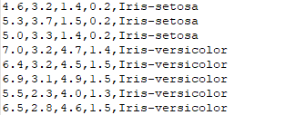
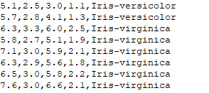
数据集样式:
import numpy as np
from matplotlib import colors
from sklearn import svm
from sklearn import model_selection
import matplotlib.pyplot as plt
import matplotlib as mpl
具体模块下载如果出现问题可见博客:
手把手教你进行pip换源
(1) 从指定路径下加载数据,将字符串转为整型
(2) 对加载的数据进行数据分割,x_train,x_test,y_train,y_test分别表示训练集特征、训练集标签、测试集特征、测试集标签
(3) 一部分数据用于构建模型,叫做训练数据,另一部分用于评估模型性能,叫做测试数据。利用scikit-learn中的train_test_split函数可以实现这个功能
# 将字符串转为整型,便于数据加载
def iris_type(s):
    it = {b'Iris-setosa':0, b'Iris-versicolor':1, b'Iris-virginica':2}
    return it[s]
# 加载数据
data_path = 'iris.data'                                     # 数据文件的路径
data = np.loadtxt(data_path,                                # 数据文件路径
                  dtype=float,                              # 数据类型
                  delimiter=',',                            # 数据分隔符
                  converters={4: iris_type})                 # 将第5列使用函数iris_type进行转换
# 数据分割
x, y = np.split(data,                                       # 要切分的数组
                (4,),                                       # 沿轴切分的位置,第5列开始往后为y
                axis=1)                                     # 代表纵向分割,按列分割
x = x[:, 0:2]                                               # 在X中我们取前两列作为特征,为了后面的可视化。x[:,0:4]代表第一维(行)全取,第二维(列)取0~2
x_train, x_test, y_train, y_test = model_selection.train_test_split(x,              # 所要划分的样本特征集
                                                                    y,              # 所要划分的样本结果
                                                                    random_state=1, # 随机数种子
                                                                    test_size=0.3)  # 测试样本占比
SVM分类器构建
# SVM分类器构建
def classifier():
    clf = svm.SVC(C=0.5,                         #误差项惩罚系数,默认值是1
                  kernel='linear',               #线性核
                  decision_function_shape='ovr') #决策函数
    return clf
# 定义模型:SVM模型定义
clf = classifier()
C为误差项惩罚系数,默认值是1,当C越大,相当于惩罚松弛变量,希望松弛变量接近0,即对误分类的惩罚增大,趋向于对训练集全分对的情况,这样对训练集测试时准确率很高,但泛化能力弱。 C值小,对误分类的惩罚减小,允许容错,将他们当成噪声点,泛化能力较强。
kernel='linear':线性核
kenrel='rbf':高斯核
decision_function_shape:决策函数
'ovr'时,为one v rest,即一个类别与其他类别进行划分
为'ovo'时,为one v one,即将类别两两之间进行划分,用二分类的方法模拟多分类的结果。
模型训练
def train(clf,x_train,y_train):
    clf.fit(x_train,         #训练集特征向量
            y_train.ravel()) #训练集目标值
# 训练SVM模型
train(clf,x_train,y_train)
模型评估
计算均值
# 并判断a b是否相等,计算acc的均值
def show_accuracy(a, b, tip):
    acc = a.ravel() == b.ravel()
    print('%s Accuracy:%.3f' %(tip, np.mean(acc)))
打印训练集和测试集的准确率
def print_accuracy(clf,x_train,y_train,x_test,y_test):
#分别打印训练集和测试集的准确率 score(x_train,y_train):表示输出x_train,y_train在模型上的准确率
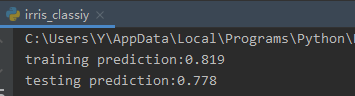
print('trianing prediction:%.3f' %(clf.score(x_train, y_train)))
print('test data prediction:%.3f' %(clf.score(x_test, y_test)))
训练集的准确率:trianing prediction:0.819
测试集的准确率:testing prediction:0.778
 # predict()表示对x_train样本进行预测,返回样本类别
show_accuracy(clf.predict(x_train), y_train, 'traing data')
show_accuracy(clf.predict(x_test), y_test, 'testing data')
训练集预测结果:training data Accuracy:0.819
测试集预测结果:testing data Accuracy:0.778
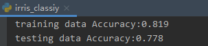
可见原始结果与预测结果是一样的
计算决策函数的值 #计算决策函数的值,表示x到各分割平面的距离
print('decision_function:\n', clf.decision_function(x_train))
模型评估
print_accuracy(clf,x_train,y_train,x_test,y_test)
输出的值
decision_function:
 [[-0.30200388  1.26702365  2.28292526]
 [ 2.1831931  -0.19913458  1.06956422]
 [ 2.25424706  0.79489006 -0.20587224]
 [ 2.22927055  0.98556708 -0.22777916]
 [ 0.95815482  2.18401419 -0.17375192]
 [ 2.23120771  0.84075865 -0.19144453]
 [ 2.17327158 -0.14884286  0.92795057]
 [-0.28667175  1.11372202  2.28302495]
 [-0.27989264  1.21274017  2.25881762]
 [-0.29313813  1.24442795  2.2732035 ]
 [-0.27008816  1.2272086   2.22682127]
 [-0.25981661  2.21998499  1.20479842]
 [-0.17071168  0.99542159  2.17180911]
 [-0.30018876  1.25829325  2.2829419 ]
 [-0.17539342  2.15368837  1.06772814]
 [ 2.25702986  0.81715893 -0.22763295]
 [-0.23988847  2.23286001  1.06656755]
 [-0.26915223  2.23333222  1.21679709]
 [ 2.22927055  0.98556708 -0.22777916]
 [ 2.2530903   0.85932358 -0.2359772 ]
 [-0.26740532  1.20784059  2.23528903]
 [ 2.26803658  0.80468578 -0.24299359]
 [-0.24030826  1.18556963  2.19011259]
 [-0.25881807  1.17240759  2.23535197]
 [-0.27273902  1.20332527  2.24866913]
 [-0.20956348  2.19674141  1.06726512]
 [-0.26556065  1.16490628  2.24871607]
 [-0.22965507  1.17870942  2.17146651]
 [ 2.25807657 -0.22526231  0.80881977]
 [-0.27322701  2.25917947  1.17077691]
 [-0.26638767  1.21631409  2.22685842]
 [-0.26740532  1.20784059  2.23528903]
 [-0.12135744  2.22922779  0.79343961]
 [-0.2365929   1.12219635  2.21706342]
 [-0.21558048  2.22640865  0.92573306]
 [ 2.22344499 -0.19955645  0.88288227]
 [ 2.22671228  0.93600592 -0.21794279]
 [ 2.26578978 -0.24701281  0.82742467]
 [-0.26556065  1.16490628  2.24871607]
 [ 2.26204658  0.89725133 -0.25453765]
 [-0.2518152   2.22343258  1.17120859]
 [-0.27340098  1.23624732  2.22678409]
 [-0.21624631  2.17118121  1.14723861]
 [ 2.22874494 -0.17513313  0.8269183 ]
 [ 2.2211989   0.87213971 -0.19151045]
 [-0.23391072  2.21566697  1.11400955]
 [ 2.22671228  0.93600592 -0.21794279]
 [-0.29609931  1.25285329  2.27596663]
 [-0.25476857  1.20746943  2.20485252]
 [-0.29672783  1.24461331  2.28083131]
 [-0.27578664  1.21663499  2.24864564]
 [-0.28091389  2.25930846  1.21661886]
 [-0.21369288  1.05233452  2.20512234]
 [-0.27669555  1.12529292  2.27023906]
 [-0.16942442  2.17056098  0.99533295]
 [ 2.24933086 -0.25468768  1.0709247 ]
 [-0.23391072  2.21566697  1.11400955]
 [ 2.18638944  1.20994285 -0.24936796]
 [-0.22656825  2.23557826  0.92551338]
 [-0.27989264  1.21274017  2.25881762]
 [ 2.24156015  0.83211053 -0.20597859]
 [-0.28390119  1.23920595  2.25400509]
 [ 2.24837463  0.81114157 -0.20592544]
 [ 2.25702986  0.81715893 -0.22763295]
 [-0.22765797  1.07419821  2.21710769]
 [-0.18996302  2.19089984  0.99497945]
 [-0.27357394  1.19278157  2.25408746]
 [ 2.23355717  0.86019975 -0.2060317 ]
 [ 2.25277813 -0.21394322  0.80875361]
 [-0.18611572  1.10670475  2.14746524]
 [ 2.25454797  0.88341904 -0.24307373]
 [-0.23391072  2.21566697  1.11400955]
 [ 2.23794605  0.91585392 -0.22774264]
 [-0.26740532  1.20784059  2.23528903]
 [ 2.0914977   1.20089769 -0.21820392]
 [ 2.25962348  0.84878847 -0.24304703]
 [-0.25213485  1.16423702  2.22696973]
 [ 2.26725005  0.88232062 -0.25923379]
 [-0.14201734  2.14344591  0.99568721]
 [ 2.25731     0.95572321 -0.25455798]
 [-0.22656825  2.23557826  0.92551338]
 [-0.19708433  2.25161696  0.79328185]
 [ 2.23957622  0.81769302 -0.19137855]
 [ 2.21575566  1.0173258  -0.21798639]
 [ 1.02668315  2.21468275 -0.21824732]
 [ 2.27472592  0.77777882 -0.24294008]
 [-0.21624631  2.17118121  1.14723861]
 [-0.24730284  1.20252603  2.19004536]
 [ 2.24156015  0.83211053 -0.20597859]
 [-0.27273902  1.20332527  2.24866913]
 [-0.19455078  2.17814555  1.06749683]
 [-0.28027257  2.2623408   1.20447285]
 [-0.28054312  1.20372124  2.26304729]
 [-0.23391072  2.21566697  1.11400955]
 [ 2.17896853 -0.12686338  0.8824238 ]
 [ 2.19820639  1.04471124 -0.20619077]
 [-0.26313706  2.23602532  1.18984329]
 [-0.25331913  2.21599142  1.18997806]
 [-0.28966527  1.23403227  2.27016072]
 [-0.23157808  2.22314802  1.06680048]
 [-0.26533811  1.22371567  2.21684157]
 [-0.25751543  1.18608093  2.22693265]
 [-0.27562627  2.24825903  1.21670804]
 [-0.27273902  1.20332527  2.24866913]
 [ 2.22671228  0.93600592 -0.21794279]]
模型使用
沿着新的轴加入一系列数组
    grid_test = np.stack((x1.flat, x2.flat), axis=1)
    print('grid_test:\n', grid_test)
输出结果:
沿着新的轴加入一系列数组:
 [[4.3       2.       ]
 [4.3       2.0120603]
 [4.3       2.0241206]
 ...
 [7.9       4.3758794]
 [7.9       4.3879397]
 [7.9       4.4      ]]
得到输出样本到决策面的距离
    z = clf.decision_function(grid_test)
    print('样本到决策面的距离:\n', z)
结果:
样本到决策面的距离:
 [[ 2.17689921  1.23467171 -0.25941323]
 [ 2.17943684  1.23363096 -0.25941107]
 [ 2.18189345  1.23256802 -0.25940892]
 ...
 [-0.27958977  0.83621535  2.28683228]
 [-0.27928358  0.8332275   2.28683314]
 [-0.27897389  0.83034313  2.28683399]]
得到预测分类值
grid_hat = clf.predict(grid_test)  # 预测分类值 得到【0,0.。。。2,2,2】
    print('预测分类值:\n', grid_hat)
    grid_hat = grid_hat.reshape(x1.shape)  # reshape grid_hat和x1形状一致
结果:
预测分类值:
 [0. 0. 0. ... 2. 2. 2.]
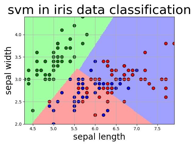
画出模型分类图
    plt.pcolormesh(x1, x2, grid_hat, cmap=cm_light)
    plt.scatter(x[:, 0], x[:, 1], c=np.squeeze(y), edgecolor='k', s=50, cmap=cm_dark)  # 样本点
    plt.scatter(x_test[:, 0], x_test[:, 1], s=120, facecolor='none', zorder=10)  # 测试点
    plt.xlabel(iris_feature[0], fontsize=20)
    plt.ylabel(iris_feature[1], fontsize=20)
    plt.xlim(x1_min, x1_max)
    plt.ylim(x2_min, x2_max)
    plt.title('svm in iris data classification', fontsize=30)
    plt.grid()
    plt.show()
 原创文章 54获赞 107访问量 1万+
关注
私信
展开阅读全文
原创文章 54获赞 107访问量 1万+
关注
私信
展开阅读全文
作者:ywsydwsbn