卷积神经网络认知及MNIST实践步骤+Kears建模对比
有关卷积神经网络的定义,以及基础理论知识在同仁的博客中写的很到位,可以参见其他博客,阅读本博客之前,请先熟知卷积神经网络的结构,基本概念及运行机理。本次写作目的主要是从应用的视角来介绍CNN,归纳实现CNN的步骤,并以MNIST为例。此外,为了加深理解和迁移,还对比了Keras建立CNN的步骤。
本文的写作也借鉴了大量博客,在此郑重感谢。
目前大多博客主对CNN的代码解析大多是基于16年左右网络代码就行解读,大同小异,删删减减。先以最为普遍的代码为例,总结建立CNN的步骤,之后再对比Keras建立CNN步骤,不难看不两种的步骤基本差不多。
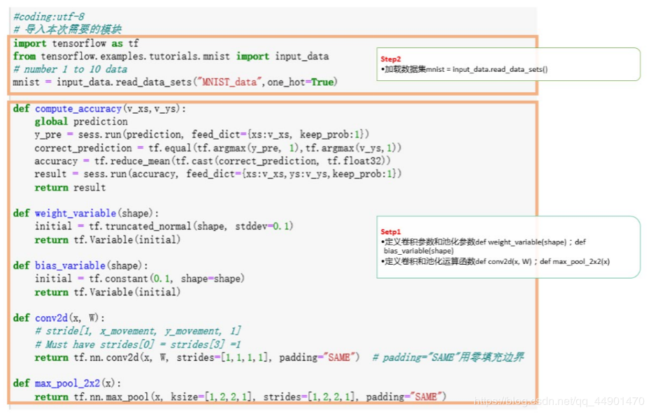
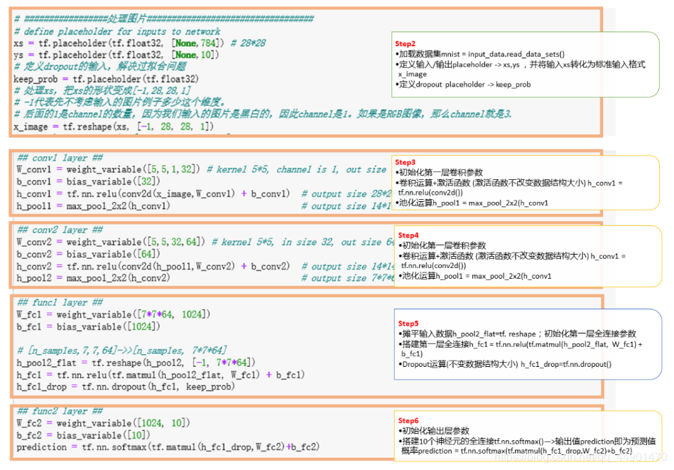
第一部分 以TF自带函数建立CNN实现MNIST识别 自定义功能函数建立CNN正如上文介绍,以网路上最为普遍的代码CNN识别MNIST进行了总结,建立两层CNN一种有八个步骤,从Step1 - > Step8,
每个步骤的主要工作和数据结构请见下图,为了便于理解,在代码截图上做了标识。
为了更好了解CNN,可以尝试在代码基础上自行摸索,如:
更改卷积核大小和深度,查看识别效果;
更改polling层参数,查看识别效果;
增加卷积层,pooling层个数,查看识别效果;
——

使用TF实现CNN识别MNIST第一种代码如下:
参见:https://blog.csdn.net/program_developer/article/details/80369989
#coding:utf-8
# 导入本次需要的模块
import tensorflow as tf
from tensorflow.examples.tutorials.mnist import input_data
# number 1 to 10 data
mnist = input_data.read_data_sets("MNIST_data",one_hot=True)
def compute_accuracy(v_xs,v_ys):
global prediction
y_pre = sess.run(prediction, feed_dict={xs:v_xs, keep_prob:1})
correct_prediction = tf.equal(tf.argmax(y_pre, 1),tf.argmax(v_ys,1))
accuracy = tf.reduce_mean(tf.cast(correct_prediction, tf.float32))
result = sess.run(accuracy, feed_dict={xs:v_xs,ys:v_ys,keep_prob:1})
return result
def weight_variable(shape):
initial = tf.truncated_normal(shape, stddev=0.1)
return tf.Variable(initial)
def bias_variable(shape):
initial = tf.constant(0.1, shape=shape)
return tf.Variable(initial)
def conv2d(x, W):
# stride[1, x_movement, y_movement, 1]
# Must have strides[0] = strides[3] =1
return tf.nn.conv2d(x, W, strides=[1,1,1,1], padding="SAME") # padding="SAME"用零填充边界
def max_pool_2x2(x):
return tf.nn.max_pool(x, ksize=[1,2,2,1], strides=[1,2,2,1], padding="SAME")
# #################处理图片##################################
# define placeholder for inputs to network
xs = tf.placeholder(tf.float32, [None,784]) # 28*28
ys = tf.placeholder(tf.float32, [None,10])
# 定义dropout的输入,解决过拟合问题
keep_prob = tf.placeholder(tf.float32)
# 处理xs,把xs的形状变成[-1,28,28,1]
# -1代表先不考虑输入的图片例子多少这个维度。
# 后面的1是channel的数量,因为我们输入的图片是黑白的,因此channel是1。如果是RGB图像,那么channel就是3.
x_image = tf.reshape(xs, [-1, 28, 28, 1])
# print(x_image.shape) #[n_samples, 28,28,1]
# #################处理图片##################################
## convl layer ##
W_conv1 = weight_variable([5,5,1,32]) # kernel 5*5, channel is 1, out size 32
b_conv1 = bias_variable([32])
h_conv1 = tf.nn.relu(conv2d(x_image,W_conv1) + b_conv1) # output size 28*28*32
h_pool1 = max_pool_2x2(h_conv1) # output size 14*14*32
## conv2 layer ##
W_conv2 = weight_variable([5,5,32,64]) # kernel 5*5, in size 32, out size 64
b_conv2 = bias_variable([64])
h_conv2 = tf.nn.relu(conv2d(h_pool1,W_conv2) + b_conv2) # output size 14*14*64
h_pool2 = max_pool_2x2(h_conv2) # output size 7*7*64
## funcl layer ##
W_fc1 = weight_variable([7*7*64, 1024])
b_fc1 = bias_variable([1024])
# [n_samples,7,7,64]->>[n_samples, 7*7*64]
h_pool2_flat = tf.reshape(h_pool2, [-1, 7*7*64])
h_fc1 = tf.nn.relu(tf.matmul(h_pool2_flat, W_fc1) + b_fc1)
h_fc1_drop = tf.nn.dropout(h_fc1, keep_prob)
## func2 layer ##
W_fc2 = weight_variable([1024, 10])
b_fc2 = bias_variable([10])
prediction = tf.nn.softmax(tf.matmul(h_fc1_drop,W_fc2)+b_fc2)
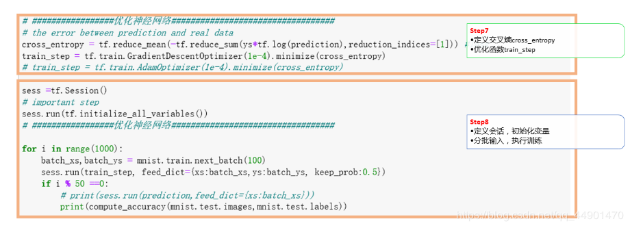
# #################优化神经网络##################################
# the error between prediction and real data
cross_entropy = tf.reduce_mean(-tf.reduce_sum(ys*tf.log(prediction),reduction_indices=[1])) #loss
train_step = tf.train.GradientDescentOptimizer(1e-4).minimize(cross_entropy)
# train_step = tf.train.AdamOptimizer(1e-4).minimize(cross_entropy)
sess =tf.Session()
# important step
sess.run(tf.initialize_all_variables())
# #################优化神经网络##################################
for i in range(1000):
batch_xs,batch_ys = mnist.train.next_batch(100)
sess.run(train_step, feed_dict={xs:batch_xs,ys:batch_ys, keep_prob:0.5})
if i % 50 ==0:
# print(sess.run(prediction,feed_dict={xs:batch_xs}))
print(compute_accuracy(mnist.test.images,mnist.test.labels))
除了以上网络常见代码外,另一种是以TF自带API函数建立CNN,整个过程大多使用结构话语句,简单明了,易于理解,不用自定义功能函数,完全调用,如下,参考博客:https://blog.csdn.net/hy13684802853/article/details/79603729
# -*- coding=utf-8 -*-
import numpy as np
import tensorflow as tf
#下载并载入MNIST手写数字库(55000*28*28)55000张训练图像
from tensorflow .examples.tutorials.mnist import input_data
#one_hot独热码的编码(encoding)形式
#0,1,2到9的10个数字
# 0 表示为0 : 1000000000
# 1 表示为1 : 0100000000
# 2 表示为2 : 0010000000等以此类推
mnist = input_data.read_data_sets('MNIST_data',one_hot=True)
#输入图片为28*28
#None表示张量(Tensor)的第一个维度可以是任何长度
input_x = tf.placeholder(tf.float32,[None,28*28])
#输出为10个数字
output_y = tf.placeholder(tf.int32,[None,10])
#改变矩阵维度,-1表示根据实际情况而定 1表示图片深度,改变形状之后的输入
images = tf.reshape(input_x,[-1,28,28,1])
#从Test数据集里选取3000个手写数字的图片和对应标签
test_x = mnist.test.images[:3000]#测试图片
test_y = mnist.test.labels[:3000]#测试标签
#构建卷积神经网络
#第一层卷积
conv1 = tf.layers.conv2d(inputs=images,
                         filters=6,
                         kernel_size=[5,5],
                         strides=1,
                         padding='same',
                         activation=tf.nn.relu
                         )#输入的形状是32*32(图片外围加入了两行0),输出的形状是28*28
#第一层池化
pool1 = tf.layers.max_pooling2d(inputs=conv1,
                                pool_size=[2,2],
                                strides=2
                                )#形状变为[14*14,32]
#第二层卷积
conv2 = tf.layers.conv2d(inputs=pool1,
                         filters=16,
                         kernel_size=[5,5],
                         strides=1,
                         activation=tf.nn.relu)#形状变为[10*10,6]
#第二层池化
pool2 = tf.layers.max_pooling2d(inputs=conv2,
                                pool_size=[2,2],
                                strides=2
                                )#形状变为[5*5,6]
conv3 = tf.layers.conv2d(inputs=pool2,
                         filters=120,
                         kernel_size=[5,5],
                         strides=1,
                         activation=tf.nn.relu)
#平坦化
flat = tf.reshape(conv3,[-1,1*1*120])
#经过全连接层
dense = tf.layers.dense(inputs=flat,
                        units=1024,
                        activation=tf.nn.relu)
#dropout 丢弃50%
dropout = tf.layers.dropout(inputs=dense,rate=0.5)
#10个神经元的全连接层,不用激励函数来做非线性化
logits = tf.layers.dense(inputs=dropout,units=10)
#计算误差,再用softmax计算百分比概率
loss = tf.losses.softmax_cross_entropy(onehot_labels=output_y,
                                       logits=logits)
#用一个Adam优化器来最小化误差,学习率设为0.001
#train_op = tf.train.AdamOptimizer(learning_rate=0.001.minimize(loss))
train_op = tf.train.AdamOptimizer(0.001).minimize(loss)
#计算与测试值和实际值的匹配程度
#返回(accuracy,update_op),会创建两个局部变量
accuracy = tf.metrics.accuracy(labels=tf.argmax(output_y,axis=1),
                               predictions=tf.argmax(logits,axis=1),)[1]
#创建会话
sess = tf.Session()
#初始化变量,全局和局部
init = tf.group(tf.global_variables_initializer(),tf.local_variables_initializer())
sess.run(init)
for x in range(2000):
    batch = mnist.train.next_batch(50) #从train数据集里去下一个50个样本
    train_loss,train_op_ = sess.run([loss,train_op],{input_x:batch[0],output_y:batch[1]})
    if x % 100 == 0:#每100轮输出一次
        test_accuracy = sess.run(accuracy,{input_x:test_x,output_y:test_y})
        print("step=%d,train loss = %.4f,test accuracy = %.2f" % (x,train_loss,test_accuracy))
#测试,打印20个测试值和真实值的对
test_output = sess.run(logits,{input_x:test_x[:20]})
inferenced_y = np.argmax(test_output,1)
print(inferenced_y,'inferenced numbers')#推测的数字
print(np.argmax(test_y[:20],1),'real numbers')#真实的数字
第二部分 Keras创建CNN
Keras中文帮助文档 https://keras-cn.readthedocs.io/en/latest/layers/convolutional_layer/
#加载数据集
from keras.datasets import mnist
(x_train,y_train),(x_test,y_test) = mnist.load_data('mnist/mnist.npz')
#print(x_train.shape,type(x_train))
#print(y_train.shape,type(y_train))
#-----------------------数据集规范化--------------------------#
from keras import backend as K
img_rows,img_cols = 28,28
#设置通道格式,默认为channels_last
if K.image_data_format() == 'channels_first':
    x_train = x_train.reshape(x_train.shape[0],1,img_rows,img_cols)
    x_test = x_test.reshape(x_test.shape[0],1,img_rows,img_cols)
    input_shape = (1,img_rows,img_cpls)
else:
    x_train = x_train.reshape(x_train.shape[0],img_rows,img_cols,1)
    x_test = x_test.reshape(x_test.shape[0],img_rows,img_cols,1)
    input_shape = (img_rows,img_cols,1)
#print(x_train.shape,type(x_train))
#print(x_test.shape,type(x_test))
#将数据类型转换为float32
X_train = x_train.astype('float32')
X_test = x_test.astype('float32')
#数据归一化
X_train /= 255
X_test /=255
#print(X_train.shape)
#print(X_test.shape)
#-----------------统统计训练数据标签数量-----------------#
import numpy as np
import matplotlib.pyplot as plt
label,count = np.unique(y_train,return_counts=True)
print(label,count)
#可视化标签
fig = plt.figure()
plt.bar(label,count,width=0.7,align='center')
plt.title('label dis')
plt.ylabel('count')
plt.xlabel('label')
plt.xticks(label)
plt.ylim(0,7500)
for a,b in zip(label,count):
    plt.text(a,b,'%d' % b,ha='center',va='bottom',fontsize=10)
plt.show()
#--------------------One-Hot编码-----------------------#
from keras.utils import np_utils
n_classes = 10
print('shape before onr-hot encoding: ',y_train.shape)
Y_train = np_utils.to_categorical(y_train,n_classes)
print('shape after one-hot encoding:',Y_train)
Y_test = np_utils.to_categorical(y_test,n_classes)
#----------使用keras sequential model定义MNIST CNN网络-------------#
from keras.models import Sequential
from keras.layers import Dense, Dropout, Flatten
from keras.layers import Conv2D, MaxPooling2D
model = Sequential()
#第一层卷积,32个3x3的卷积核,激活函数使用relu
model.add(Conv2D(filters=32,kernel_size=(3,3),activation='relu',input_shape=input_shape))
#第二层卷积,64个3x3的卷积核,激活函数使用relu
model.add(Conv2D(filters=64,kernel_size=(3,3),activation='relu'))
#最大池化曾,池化窗口2x2
model.add(MaxPooling2D(pool_size=(2,2)))
#Dropout 25%的输入神经元
model.add(Dropout(0.25))
#将pooled feature map摊平后输入全链接层
model.add(Flatten())
#全连接层
model.add(Dense(128,activation='relu'))
#Dropout 50%的输入神经元
model.add(Dropout(0.5))
#使用softmax 激活函数做多分类,输出数字的概率
model.add(Dense(n_classes,activation='softmax'))
#-------------查看MNIST CNN模型网络结构---------------#
model.summary()#表格形式显示每层网络的output的数据结构,及参数量
#获取每层形状
for layer in model.layers:
    print(layer.get_output_at(0).get_shape().as_list())
#----------------编译模型--------------------#
model.compile(loss='categorical_crossentropy',metrics=['accuracy'],optimizer='adam')
#------------训练模型,并将指标保存到history中-----------#
history = model.fit(X_train,
                   Y_train,
                   batch_size=128,
                   epochs=5,
                   verbose=2,
                   validation_data=(X_test,Y_test))
#---------------可视化指标-------------------#
fig = plt.figure()
plt.subplot(2,1,1)
plt.plot(history.history['acc'])
plt.plot(plt.plot(history.history['val_acc'])
plt.title('model acc')
plt.ylabel('acc')
plt.xlabel('epoch')
plt.legend(['train','test'],loc='lower right')
plt.subplot(2,1,2)
plt.plot(history.history['loss'])
plt.plot(plt.plot(history.history['val_loss'])
plt.title('model loss')
plt.ylabel('loss')
plt.xlabel('epoch')
plt.legend(['train','test'],loc='upper right')
plt.tight_layout()
plt.show()
#-----------保存模型---------#
#-----------加载模型---------#
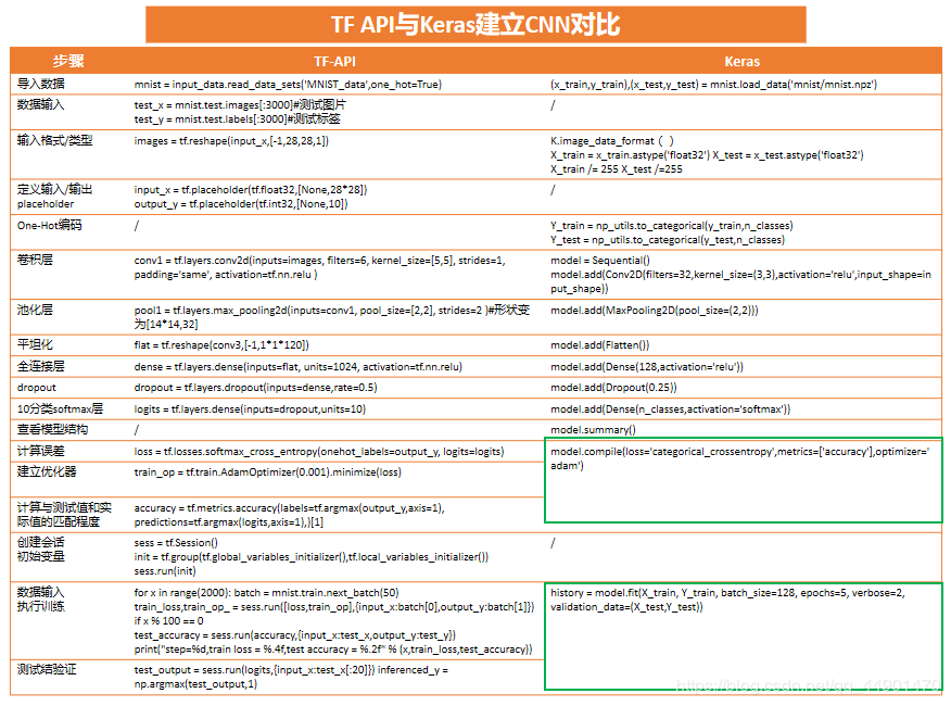
Tensorflow与Keras建立CNN对比
通过以上建立CNN实现MNIST的三段代码的可读性,结构性,编译性,不难看出使用Keras与TF自带的API建立CNN为优先选择。TF-API与Keras建模过程对比结果如下图:
以下几点比较明显
参考博客如下:
CNN参数计算及不同CNN的结构:
https://blog.csdn.net/qian99/article/details/79008053
https://www.cnblogs.com/touch-skyer/p/9150039.html
CNN介绍 - 分割图片 https://www.leiphone.com/news/201705/6Zi5evpIaKJRHsJj.html
MINST 代码介绍 https://blog.csdn.net/program_developer/article/details/80369989
系统介绍CNN https://blog.csdn.net/cxmscb/article/details/71023576?depth_1-utm_source=distribute.pc_relevant.none-task&utm_source=distribute.pc_relevant.none-task
结构参数选择https://blog.csdn.net/ts719796895/article/details/95043540
http://danielnouri.org/notes/2014/12/17/using-convolutional-neural-nets-to-detect-facial-keypoints-tutorial/?spm=a2c4e.10696291.0.0.748319a4oLMWRv
认识卷积核 https://segmentfault.com/q/1010000016667038
作者:午后看晴