经典卷积神经网络模型—AlexNet，VGG，GoogLeNet

Vanessa ·

更新时间:2024-09-20

· 855 次阅读

AlexNet

特征

8层变换，其中有5层卷积和2层全连接隐藏层，以及1个全连接输出层。将sigmoid激活函数改成了更加简单的ReLU激活函数。用Dropout来控制全连接层的模型复杂度。引入数据增强，如翻转、裁剪和颜色变化，从而进一步扩大数据集来缓解过拟合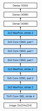
在这里插入图片描述

第一个卷积层
输入的图片大小为:2242243（或者是2272273）
第一个卷积层为:111196即尺寸为1111,有96个卷积核,步长为4,卷积层后跟ReLU,因此输出的尺寸为 224/4=56,去掉边缘为55,因此其输出的每个feature map 为 555596,同时后面跟LRN层,尺寸不变.
最大池化层,核大小为33,步长为2,因此feature map的大小为:272796.

第二层卷积层
输入的tensor为272796
卷积和的大小为: 55256,步长为1,尺寸不会改变,同样紧跟ReLU,和LRN层.
最大池化层,和大小为33,步长为2,因此feature map为:1313*256

第三层至第五层卷积层
输入的tensor为1313256
第三层卷积为 33384,步长为1,加上ReLU
第四层卷积为 33384,步长为1,加上ReLU
第五层卷积为 33256,步长为1,加上ReLU
第五层后跟最大池化层,核大小33,步长为2,因此feature map:66*256

第六层至第八层全连接层
接下来的三层为全连接层,分别为:
FC : 4096 + ReLU
FC:4096 + ReLU
FC: 1000 最后一层为softmax为1000类的概率值.

本文中的模型都是在FashionMNIST数据集上验证
AlexNet模型pytorch实现

import time
import torch
from torch import nn, optim
import torchvision
import numpy as np
import sys
sys.path.append("/home/") 
import os
import torch.nn.functional as F
device = torch.device('cuda' if torch.cuda.is_available() else 'cpu')
class AlexNet(nn.Module):
    def __init__(self):
        super(AlexNet, self).__init__()
        self.conv = nn.Sequential(
            nn.Conv2d(1, 96, 11, 4), # in_channels, out_channels, kernel_size, stride, padding
            nn.ReLU(),
            nn.MaxPool2d(3, 2), # kernel_size, stride
            # 减小卷积窗口，使用填充为2来使得输入与输出的高和宽一致，且增大输出通道数
            nn.Conv2d(96, 256, 5, 1, 2),
            nn.ReLU(),
            nn.MaxPool2d(3, 2),
            # 连续3个卷积层，且使用更小的卷积窗口。除了最后的卷积层外，进一步增大了输出通道数。
            # 前两个卷积层后不使用池化层来减小输入的高和宽
            nn.Conv2d(256, 384, 3, 1, 1),
            nn.ReLU(),
            nn.Conv2d(384, 384, 3, 1, 1),
            nn.ReLU(),
            nn.Conv2d(384, 256, 3, 1, 1),
            nn.ReLU(),
            nn.MaxPool2d(3, 2)
        )
         # 这里全连接层的输出个数比LeNet中的大数倍。使用丢弃层来缓解过拟合
        self.fc = nn.Sequential(
            nn.Linear(256*5*5, 4096),
            nn.ReLU(),
            nn.Dropout(0.5),
            #由于使用CPU镜像，精简网络，若为GPU镜像可添加该层
            nn.Linear(4096, 4096),
            nn.ReLU(),
            nn.Dropout(0.5),
            # 输出层。由于这里使用Fashion-MNIST，所以用类别数为10，而非论文中的1000
            nn.Linear(4096, 10),
        )
    def forward(self, img):
        feature = self.conv(img)
        output = self.fc(feature.view(img.shape[0], -1))
        return output
def load_data_fashion_mnist(batch_size, resize=None, root='/home/kesci/input/FashionMNIST2065'):
    """Download the fashion mnist dataset and then load into memory."""
    trans = []
    if resize:
        trans.append(torchvision.transforms.Resize(size=resize))
    trans.append(torchvision.transforms.ToTensor())
    transform = torchvision.transforms.Compose(trans)
    mnist_train = torchvision.datasets.FashionMNIST(root=root, train=True, download=True, transform=transform)
    mnist_test = torchvision.datasets.FashionMNIST(root=root, train=False, download=True, transform=transform)
    train_iter = torch.utils.data.DataLoader(mnist_train, batch_size=batch_size, shuffle=True, num_workers=2)
    test_iter = torch.utils.data.DataLoader(mnist_test, batch_size=batch_size, shuffle=False, num_workers=2)
    return train_iter, test_iter
def evaluate_accuracy(data_iter, net, device=None):
    if device is None and isinstance(net, torch.nn.Module):
        # 如果没指定device就使用net的device
        device = list(net.parameters())[0].device 
    acc_sum, n = 0.0, 0
    with torch.no_grad():
        for X, y in data_iter:
            if isinstance(net, torch.nn.Module):
                net.eval() # 评估模式, 这会关闭dropout
                acc_sum += (net(X.to(device)).argmax(dim=1) == y.to(device)).float().sum().cpu().item()
                net.train() # 改回训练模式
            else: # 自定义的模型, 3.13节之后不会用到, 不考虑GPU
                if('is_training' in net.__code__.co_varnames): # 如果有is_training这个参数
                    # 将is_training设置成False
                    acc_sum += (net(X, is_training=False).argmax(dim=1) == y).float().sum().item() 
                else:
                    acc_sum += (net(X).argmax(dim=1) == y).float().sum().item() 
            n += y.shape[0]
    return acc_sum / n    
def train(net, train_iter, test_iter, batch_size, optimizer, device, num_epochs):
    net = net.to(device)
    print("training on ", device)
    loss = torch.nn.CrossEntropyLoss()
    for epoch in range(num_epochs):
        train_l_sum, train_acc_sum, n, batch_count, start = 0.0, 0.0, 0, 0, time.time()
        for X, y in train_iter:
            X = X.to(device)
            y = y.to(device)
            y_hat = net(X)
            l = loss(y_hat, y)
            optimizer.zero_grad()
            l.backward()
            optimizer.step()
            train_l_sum += l.cpu().item()
            train_acc_sum += (y_hat.argmax(dim=1) == y).sum().cpu().item()
            n += y.shape[0]
            batch_count += 1
        test_acc = evaluate_accuracy(test_iter, net)
        print('epoch %d, loss %.4f, train acc %.3f, test acc %.3f, time %.1f sec'
              % (epoch + 1, train_l_sum / batch_count, train_acc_sum / n, test_acc, time.time() - start))
batch_size = 16
lr, num_epochs = 0.001, 3
optimizer = torch.optim.Adam(net.parameters(), lr=lr)
net = AlexNet()
print(net)
# 如出现“out of memory”的报错信息，可减小batch_size或resize
train_iter, test_iter = load_data_fashion_mnist(batch_size,224)
train(net, train_iter, test_iter, batch_size, optimizer, device, num_epochs)

VGG

VGG 是一个很经典的卷积神经网络结构，是由 AlexNet 改进的，相比于 AlexNet，主要的改变有两个地方：
1 使用 3 x 3 卷积核代替 AlexNet 中的大卷积核
2 使用 2 x 2 池化核代替 AlexNet 的 3 x 3 池化核

VGGNet 有很多类型，论文中提出了 4 种不同层次的网络结构（从 11 层到 19 层）：
在这里插入图片描述
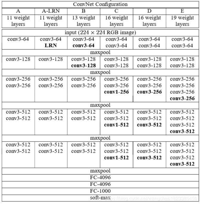
VGG 有很多优点，最本质的特点就是用小的卷积核(3x3)代替大的卷积核，2个 3x3 卷积堆叠等于1个 5x5 卷积，3 个 3x3 堆叠等于1个 7x7 卷积，感受野大小不变。

可以想象一下，在步长 s 为 1，填充 padding 为 0 时，2 个 3x3 卷积后的图像 size 为 (((N-3)/1+1)-3)/1+1 = ((N-3+1)-3+1) = N-4 = (N-5)/1+1。且做卷积后，得到的特征，都是从原图像上相同的像素点提取的（原图像每 5x5 的空域像素点对应一个新的特征），因此感受野大小不变。故 2 个 3x3 的卷积核与 5x5 的卷积核等价。

相同的效果，采用小的卷积核，可以增加网络的深度，从而引入更多的非线性（激活函数）。

下面用pytorch实现VGG11模型

import time
import torch
from torch import nn, optim
import torchvision
import numpy as np
import sys
sys.path.append("/home/") 
import os
import torch.nn.functional as F
def vgg_block(num_convs, in_channels, out_channels): #卷积层个数，输入通道数，输出通道数
    blk = []
    for i in range(num_convs):
        if i == 0:
            blk.append(nn.Conv2d(in_channels, out_channels, kernel_size=3, padding=1))
        else:
            blk.append(nn.Conv2d(out_channels, out_channels, kernel_size=3, padding=1))
        blk.append(nn.ReLU())
    blk.append(nn.MaxPool2d(kernel_size=2, stride=2)) # 这里会使宽高减半
    return nn.Sequential(*blk)
conv_arch = ((1, 1, 64), (1, 64, 128), (2, 128, 256), (2, 256, 512), (2, 512, 512))
# 经过5个vgg_block, 宽高会减半5次, 变成 224/32 = 7
fc_features = 512 * 7 * 7 # c * w * h
fc_hidden_units = 4096 # 任意
def vgg(conv_arch, fc_features, fc_hidden_units=4096):
    net = nn.Sequential()
    # 卷积层部分
    for i, (num_convs, in_channels, out_channels) in enumerate(conv_arch):
        # 每经过一个vgg_block都会使宽高减半
        net.add_module("vgg_block_" + str(i+1), vgg_block(num_convs, in_channels, out_channels))
    # 全连接层部分
    net.add_module("fc", nn.Sequential(d2l.FlattenLayer(),
                                 nn.Linear(fc_features, fc_hidden_units),
                                 nn.ReLU(),
                                 nn.Dropout(0.5),
                                 nn.Linear(fc_hidden_units, fc_hidden_units),
                                 nn.ReLU(),
                                 nn.Dropout(0.5),
                                 nn.Linear(fc_hidden_units, 10)
                                ))
    return net
#载入数据集
def load_data_fashion_mnist(batch_size, resize=None, root='/home/kesci/input/FashionMNIST2065'):
    """Download the fashion mnist dataset and then load into memory."""
    trans = []
    if resize:
        trans.append(torchvision.transforms.Resize(size=resize))
    trans.append(torchvision.transforms.ToTensor())
    transform = torchvision.transforms.Compose(trans)
    mnist_train = torchvision.datasets.FashionMNIST(root=root, train=True, download=True, transform=transform)
    mnist_test = torchvision.datasets.FashionMNIST(root=root, train=False, download=True, transform=transform)
    train_iter = torch.utils.data.DataLoader(mnist_train, batch_size=batch_size, shuffle=True, num_workers=2)
    test_iter = torch.utils.data.DataLoader(mnist_test, batch_size=batch_size, shuffle=False, num_workers=2)
    return train_iter, test_iter
def train(net, train_iter, test_iter, batch_size, optimizer, device, num_epochs):
    net = net.to(device)
    print("training on ", device)
    loss = torch.nn.CrossEntropyLoss()
    for epoch in range(num_epochs):
        train_l_sum, train_acc_sum, n, batch_count, start = 0.0, 0.0, 0, 0, time.time()
        for X, y in train_iter:
            X = X.to(device)
            y = y.to(device)
            y_hat = net(X)
            l = loss(y_hat, y)
            optimizer.zero_grad()
            l.backward()
            optimizer.step()
            train_l_sum += l.cpu().item()
            train_acc_sum += (y_hat.argmax(dim=1) == y).sum().cpu().item()
            n += y.shape[0]
            batch_count += 1
        test_acc = evaluate_accuracy(test_iter, net)
        print('epoch %d, loss %.4f, train acc %.3f, test acc %.3f, time %.1f sec'
              % (epoch + 1, train_l_sum / batch_count, train_acc_sum / n, test_acc, time.time() - start))
net = vgg(conv_arch, fc_features, fc_hidden_units)
train_iter, test_iter = load_data_fashion_mnist(batch_size,224)
batchsize=16
lr, num_epochs = 0.001, 5
optimizer = torch.optim.Adam(net.parameters(), lr=lr)
train(net, train_iter, test_iter, batch_size, optimizer, device, num_epochs)

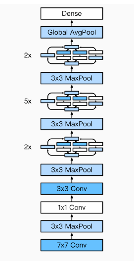
GoogLeNet
由Inception基础块组成。

Inception块相当于一个有4条线路的子网络。它通过不同窗口形状的卷积层和最大池化层来并行抽取信息，并使用1×1卷积层减少通道数从而降低模型复杂度。

可以自定义的超参数是每个层的输出通道数，我们以此来控制模型复杂度。
在这里插入图片描述

class Inception(nn.Module):
    # c1 - c4为每条线路里的层的输出通道数
    def __init__(self, in_c, c1, c2, c3, c4):
        super(Inception, self).__init__()
        # 线路1，单1 x 1卷积层
        self.p1_1 = nn.Conv2d(in_c, c1, kernel_size=1)
        # 线路2，1 x 1卷积层后接3 x 3卷积层
        self.p2_1 = nn.Conv2d(in_c, c2[0], kernel_size=1)
        self.p2_2 = nn.Conv2d(c2[0], c2[1], kernel_size=3, padding=1)
        # 线路3，1 x 1卷积层后接5 x 5卷积层
        self.p3_1 = nn.Conv2d(in_c, c3[0], kernel_size=1)
        self.p3_2 = nn.Conv2d(c3[0], c3[1], kernel_size=5, padding=2)
        # 线路4，3 x 3最大池化层后接1 x 1卷积层
        self.p4_1 = nn.MaxPool2d(kernel_size=3, stride=1, padding=1)
        self.p4_2 = nn.Conv2d(in_c, c4, kernel_size=1)
    def forward(self, x):
        p1 = F.relu(self.p1_1(x))
        p2 = F.relu(self.p2_2(F.relu(self.p2_1(x))))
        p3 = F.relu(self.p3_2(F.relu(self.p3_1(x))))
        p4 = F.relu(self.p4_2(self.p4_1(x)))
        return torch.cat((p1, p2, p3, p4), dim=1)  # 在通道维上连结输出

GoogLeNet完整模型结构
在这里插入图片描述

b1 = nn.Sequential(nn.Conv2d(1, 64, kernel_size=7, stride=2, padding=3),
                   nn.ReLU(),
                   nn.MaxPool2d(kernel_size=3, stride=2, padding=1))
b2 = nn.Sequential(nn.Conv2d(64, 64, kernel_size=1),
                   nn.Conv2d(64, 192, kernel_size=3, padding=1),
                   nn.MaxPool2d(kernel_size=3, stride=2, padding=1))
b3 = nn.Sequential(Inception(192, 64, (96, 128), (16, 32), 32),
                   Inception(256, 128, (128, 192), (32, 96), 64),
                   nn.MaxPool2d(kernel_size=3, stride=2, padding=1))
b4 = nn.Sequential(Inception(480, 192, (96, 208), (16, 48), 64),
                   Inception(512, 160, (112, 224), (24, 64), 64),
                   Inception(512, 128, (128, 256), (24, 64), 64),
                   Inception(512, 112, (144, 288), (32, 64), 64),
                   Inception(528, 256, (160, 320), (32, 128), 128),
                   nn.MaxPool2d(kernel_size=3, stride=2, padding=1))
b5 = nn.Sequential(Inception(832, 256, (160, 320), (32, 128), 128),
                   Inception(832, 384, (192, 384), (48, 128), 128),
                   d2l.GlobalAvgPool2d())
net = nn.Sequential(b1, b2, b3, b4, b5, 
                    d2l.FlattenLayer(), nn.Linear(1024, 10))
net = nn.Sequential(b1, b2, b3, b4, b5, d2l.FlattenLayer(), nn.Linear(1024, 10))
X = torch.rand(1, 1, 96, 96)
for blk in net.children(): 
    X = blk(X)
    print('output shape: ', X.shape)
#batchsize=128
batch_size = 16
# 如出现“out of memory”的报错信息，可减小batch_size或resize
#train_iter, test_iter = d2l.load_data_fashion_mnist(batch_size, resize=96)
lr, num_epochs = 0.001, 5
optimizer = torch.optim.Adam(net.parameters(), lr=lr)
train(net, train_iter, test_iter, batch_size, optimizer, device, num_epochs)

作者：一名小菜鸟的学习之路

googlenet 模型 vgg 网络模型神经网络模型卷积神经网络 alexnet 神经网络卷积