机器学习-三种回归方法（Ridge、LASSO和ElasticNet回归）

Vivienne ·

更新时间:2024-09-21

· 787 次阅读

Section I: Brief Introduction on Three Regression Models

Regulation is one approach to tackle the problem of overfitting by adding additional information, and thereby shrinking the parameter values of the model to induce a penalty against complexity. The most popular approaches to regularized linear regression are the so-called Ridge Regression, Least Absolute Shrinkage and Selection Operator(LASSO), AND Elastic Net Models.

Ridge Regression: L2 Regulation LASSO Regression: L1 Regulation ElasticNet Regression: L2 and L1 Regulation

Two Quantitative Measures

Mean Square Error(MSE) R2 Score - Standard Version of MSE

FROM
Sebastian Raschka, Vahid Mirjalili. Python机器学习第二版. 南京：东南大学出版社，2018.

第一部分：Ridge Regression
代码

from sklearn import datasets
from sklearn.model_selection import train_test_split
from sklearn.linear_model import LinearRegression
from sklearn.metrics import mean_squared_error,r2_score
import matplotlib.pyplot as plt
import warnings
warnings.filterwarnings("ignore")
plt.rcParams['figure.dpi']=200
plt.rcParams['savefig.dpi']=200
font = {'family': 'Times New Roman',
        'weight': 'light'}
plt.rc("font", **font)
#Section 1: Load data and split it into Train/Test dataset
price=datasets.load_boston()
X=price.data
y=price.target
X_train,X_test,y_train,y_test=train_test_split(X,y,
                                               test_size=0.3)
#Section 2: Ridge Regression and Least Shrinkage and Selection Operator(LASSO) AND Elastic Net
#Ridge: L2 Regulation
#LASSO: L1 Regulation
#Elastic Net: Both L1 and L2 Regulation
#Section 2.1: Ridge Model
#The parameter alpha would be the regulation stength.
from sklearn.linear_model import Ridge
ridge=Ridge(alpha=1.0)
ridge.fit(X_train,y_train)
y_train_pred=ridge.predict(X_train)
y_test_pred=ridge.predict(X_test)
plt.scatter(y_train_pred,y_train_pred-y_train,
            c='blue',marker='o',edgecolor='white',
            label='Training Data')
plt.scatter(y_test_pred,y_test_pred-y_test,
            c='limegreen',marker='s',edgecolors='white',
            label='Test Data')
plt.xlabel("Predicted Values")
plt.ylabel("The Residuals")
plt.legend(loc='upper left')
plt.hlines(y=0,xmin=-10,xmax=50,color='black',lw=2)
plt.xlim([-10,50])
plt.title("Ridge Regression Model")
plt.savefig('./fig2.png')
plt.show()
print("\nMSE Train in Ridge: %.3f, Test: %.3f" % \
      (mean_squared_error(y_train,y_train_pred),
       mean_squared_error(y_test,y_test_pred)))
print("R^2 Train in Ridge: %.3f, Test: %.3f" % \
      (r2_score(y_train,y_train_pred),
       r2_score(y_test,y_test_pred)))

结果
在这里插入图片描述
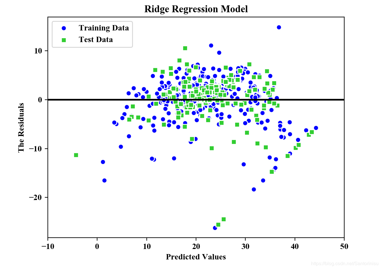
预测精度：

MSE Train in Ridge: 20.889, Test: 25.470
R^2 Train in Ridge: 0.739, Test: 0.728

第二部分：LASSO Regression

在第一部分的基础上，进一步添加如下代码。
代码

#Section 2.2: LASSO Model
#The parameter alpha would be the regulation stength.
from sklearn.linear_model import Lasso
lasso=Lasso(alpha=1.0)
lasso.fit(X_train,y_train)
y_train_pred=lasso.predict(X_train)
y_test_pred=lasso.predict(X_test)
plt.scatter(y_train_pred,y_train_pred-y_train,
            c='blue',marker='o',edgecolor='white',
            label='Training Data')
plt.scatter(y_test_pred,y_test_pred-y_test,
            c='limegreen',marker='s',edgecolors='white',
            label='Test Data')
plt.xlabel("Predicted Values")
plt.ylabel("The Residuals")
plt.legend(loc='upper left')
plt.hlines(y=0,xmin=-10,xmax=50,color='black',lw=2)
plt.xlim([-10,50])
plt.title("LASSO Regression Model")
plt.savefig('./fig3.png')
plt.show()
print("\nMSE Train in LASSO: %.3f, Test: %.3f" % \
      (mean_squared_error(y_train,y_train_pred),
       mean_squared_error(y_test,y_test_pred)))
print("R^2 Train in LASSO: %.3f, Test: %.3f" % \
      (r2_score(y_train,y_train_pred),
       r2_score(y_test,y_test_pred)))

结果
在这里插入图片描述
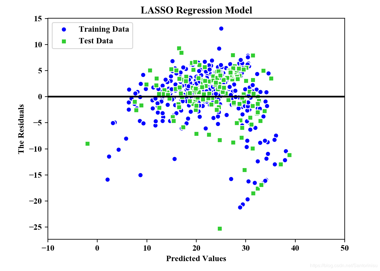
预测精度：

MSE Train in LASSO: 25.618, Test: 32.727
R^2 Train in LASSO: 0.680, Test: 0.650

第三部分：ElasticNet Regression

在第一、二部分的基础上，进一步添加如下代码。
代码

#Section 2.3: Elastic Net Model
#The parameter alpha would be the regulation stength.
from sklearn.linear_model import ElasticNet
elastic_net=ElasticNet(alpha=1.0,l1_ratio=0.5)
elastic_net.fit(X_train,y_train)
y_train_pred=elastic_net.predict(X_train)
y_test_pred=elastic_net.predict(X_test)
plt.scatter(y_train_pred,y_train_pred-y_train,
            c='blue',marker='o',edgecolor='white',
            label='Training Data')
plt.scatter(y_test_pred,y_test_pred-y_test,
            c='limegreen',marker='s',edgecolors='white',
            label='Test Data')
plt.xlabel("Predicted Values")
plt.ylabel("The Residuals")
plt.legend(loc='upper left')
plt.hlines(y=0,xmin=-10,xmax=50,color='black',lw=2)
plt.xlim([-10,50])
plt.title("ElasticNet Regression Model")
plt.savefig('./fig4.png')
plt.show()
print("\nMSE Train in ElasticNet: %.3f, Test: %.3f" % \
      (mean_squared_error(y_train,y_train_pred),
       mean_squared_error(y_test,y_test_pred)))
print("R^2 Train in ElasticNet: %.3f, Test: %.3f" % \
      (r2_score(y_train,y_train_pred),
       r2_score(y_test,y_test_pred)))

结果
在这里插入图片描述
预测精度：

MSE Train in ElasticNet: 24.999, Test: 31.943
R^2 Train in ElasticNet: 0.688, Test: 0.659

参考文献
Sebastian Raschka, Vahid Mirjalili. Python机器学习第二版. 南京：东南大学出版社，2018.

附录

from sklearn import datasets
from sklearn.model_selection import train_test_split
from sklearn.linear_model import LinearRegression
from sklearn.metrics import mean_squared_error,r2_score
import matplotlib.pyplot as plt
import warnings
warnings.filterwarnings("ignore")
plt.rcParams['figure.dpi']=200
plt.rcParams['savefig.dpi']=200
font = {'family': 'Times New Roman',
        'weight': 'light'}
plt.rc("font", **font)
#Section 1: Load data and split it into Train/Test dataset
price=datasets.load_boston()
X=price.data
y=price.target
X_train,X_test,y_train,y_test=train_test_split(X,y,
                                               test_size=0.3)
#Section 2: Ridge Regression and Least Shrinkage and Selection Operator(LASSO) AND Elastic Net
#Ridge: L2 Regulation
#LASSO: L1 Regulation
#Elastic Net: Both L1 and L2 Regulation
#Section 2.1: Ridge Model
#The parameter alpha would be the regulation stength.
from sklearn.linear_model import Ridge
ridge=Ridge(alpha=1.0)
ridge.fit(X_train,y_train)
y_train_pred=ridge.predict(X_train)
y_test_pred=ridge.predict(X_test)
plt.scatter(y_train_pred,y_train_pred-y_train,
            c='blue',marker='o',edgecolor='white',
            label='Training Data')
plt.scatter(y_test_pred,y_test_pred-y_test,
            c='limegreen',marker='s',edgecolors='white',
            label='Test Data')
plt.xlabel("Predicted Values")
plt.ylabel("The Residuals")
plt.legend(loc='upper left')
plt.hlines(y=0,xmin=-10,xmax=50,color='black',lw=2)
plt.xlim([-10,50])
plt.title("Ridge Regression Model")
plt.savefig('./fig2.png')
plt.show()
print("\nMSE Train in Ridge: %.3f, Test: %.3f" % \
      (mean_squared_error(y_train,y_train_pred),
       mean_squared_error(y_test,y_test_pred)))
print("R^2 Train in Ridge: %.3f, Test: %.3f" % \
      (r2_score(y_train,y_train_pred),
       r2_score(y_test,y_test_pred)))
#Section 2.2: LASSO Model
#The parameter alpha would be the regulation stength.
from sklearn.linear_model import Lasso
lasso=Lasso(alpha=1.0)
lasso.fit(X_train,y_train)
y_train_pred=lasso.predict(X_train)
y_test_pred=lasso.predict(X_test)
plt.scatter(y_train_pred,y_train_pred-y_train,
            c='blue',marker='o',edgecolor='white',
            label='Training Data')
plt.scatter(y_test_pred,y_test_pred-y_test,
            c='limegreen',marker='s',edgecolors='white',
            label='Test Data')
plt.xlabel("Predicted Values")
plt.ylabel("The Residuals")
plt.legend(loc='upper left')
plt.hlines(y=0,xmin=-10,xmax=50,color='black',lw=2)
plt.xlim([-10,50])
plt.title("LASSO Regression Model")
plt.savefig('./fig3.png')
plt.show()
print("\nMSE Train in LASSO: %.3f, Test: %.3f" % \
      (mean_squared_error(y_train,y_train_pred),
       mean_squared_error(y_test,y_test_pred)))
print("R^2 Train in LASSO: %.3f, Test: %.3f" % \
      (r2_score(y_train,y_train_pred),
       r2_score(y_test,y_test_pred)))
#Section 2.3: Elastic Net Model
#The parameter alpha would be the regulation stength.
from sklearn.linear_model import ElasticNet
elastic_net=ElasticNet(alpha=1.0,l1_ratio=0.5)
elastic_net.fit(X_train,y_train)
y_train_pred=elastic_net.predict(X_train)
y_test_pred=elastic_net.predict(X_test)
plt.scatter(y_train_pred,y_train_pred-y_train,
            c='blue',marker='o',edgecolor='white',
            label='Training Data')
plt.scatter(y_test_pred,y_test_pred-y_test,
            c='limegreen',marker='s',edgecolors='white',
            label='Test Data')
plt.xlabel("Predicted Values")
plt.ylabel("The Residuals")
plt.legend(loc='upper left')
plt.hlines(y=0,xmin=-10,xmax=50,color='black',lw=2)
plt.xlim([-10,50])
plt.title("ElasticNet Regression Model")
plt.savefig('./fig4.png')
plt.show()
print("\nMSE Train in ElasticNet: %.3f, Test: %.3f" % \
      (mean_squared_error(y_train,y_train_pred),
       mean_squared_error(y_test,y_test_pred)))
print("R^2 Train in ElasticNet: %.3f, Test: %.3f" % \
      (r2_score(y_train,y_train_pred),
       r2_score(y_test,y_test_pred)))

作者：Santorinisu

lasso 方法学习回归机器学习

1024 个赞