动手学深度学习PyTorch版 | (3)过拟合、欠拟合及其解决方案
训练模型中经常出现的两类典型问题:
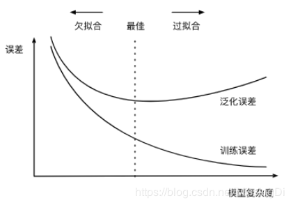
欠拟合:模型无法得到较低的训练误差 过拟合:模型的训练误差远小于它在测试数据集上的误差在实践中,我们要尽可能同时应对欠拟合和过拟合。有很多因素可能导致这两种拟合问题,在这里我们重点讨论两个因素:模型复杂度和训练数据集大小。
- 模型复杂度
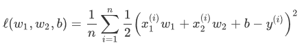
为了解释模型复杂度,我们以多项式函数拟合为例。给定一个由标量数据特征 x 和对应的标量标签 y 组成的训练数据集,多项式函数拟合的目标是找一个K阶多项式函数:
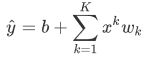
来近似 y。在上式中,wkw_kwk是模型的权重参数,b是偏差参数。与线性回归相同,多项式函数拟合也使用平方损失函数。特别地,一阶多项式函数拟合又叫线性函数拟合。
给定训练数据集,模型复杂度和误差之间的关系:
- 训练数据集大小
影响欠拟合和过拟合的另一个重要因素是训练数据集的大小。一般来说,如果训练数据集中样本数过少,特别是比模型参数数量(按元素计)更少时,过拟合更容易发生。此外,泛化误差不会随训练数据集里样本数量增加而增大。因此,在计算资源允许的范围之内,我们通常希望训练数据集大一些,特别是在模型复杂度较高时,例如层数较多的深度学习模型。
下面以多项式函数拟合实验为例,进行训练并实例演示欠拟合和过拟合。
二、多项式函数拟合实验引入实验需要的包
import torch
import numpy as np
import sys
sys.path.append("/home/kesci/input")
import d2lzh1981 as d2l
print(torch.__version__)
2.1 初始化模型参数
n_train, n_test,true_w,true_b = 100,100,[1.2,-3.4,5.6], 5
features = torch.randn((n_train + n_test, 1))
print(features.shape)
poly_features = torch.cat((features,torch.pow(features,2),torch.pow(features,3)),1)  # cat()为连接操作,连接维度为列(1);pow()为张量的幂操作
print(poly_features.shape)
labels = (true_w[0] * poly_features[:, 0] + true_w[1] * poly_features[:, 1]
          + true_w[2] * poly_features[:, 2] + true_b)
labels += torch.tensor(np.random.normal(0, 0.01, size=labels.size()), dtype=torch.float)  # 添加噪声
![]()
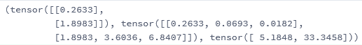
features[:2],poly_features[:2],labels[:2]
def semilogy(x_vals, y_vals, x_label, y_label, x2_vals=None, y2_vals=None,
             legend=None, figsize=(3.5, 2.5)):
    d2l.plt.xlabel(x_label)
    d2l.plt.ylabel(y_label)
    d2l.plt.semilogy(x_vals, y_vals)
    if x2_vals and y2_vals:
        d2l.plt.semilogy(x2_vals, y2_vals, linestyle=':')
        d2l.plt.legend(legend)
num_epochs, loss = 100, torch.nn.MSELoss()
def fit_and_plot(train_features, test_features, train_labels, test_labels):
# 初始化网络模型
print('train_features.shape',train_features.shape)
print(('train_features.shape[-1]',train_features.shape[-1]))
net = torch.nn.Linear(train_features.shape[-1], 1) #train_features.shape[-1]为3
# 通过Linear文档可知,pytorch已经将参数初始化了,所以我们这里就不手动初始化了
# 设置批量大小
print('train_labels.shape[0]',train_labels.shape[0])
batch_size = min(10, train_labels.shape[0])
dataset = torch.utils.data.TensorDataset(train_features, train_labels) # 设置数据集,大概意思是整合x和y,使其对应。即x的每一行对应y的每一行
train_iter = torch.utils.data.DataLoader(dataset, batch_size, shuffle=True) # 设置获取数据方式
optimizer = torch.optim.SGD(net.parameters(), lr=0.01) # 设置优化函数,使用的是随机梯度下降优化
train_ls, test_ls = [], []
for _ in range(num_epochs):
for X, y in train_iter: # 取一个批量的数据
l = loss(net(X), y.view(-1, 1)) # 输入到网络中计算输出,并和标签比较求得损失函数
optimizer.zero_grad() # 梯度清零,防止梯度累加干扰优化
l.backward() # 求梯度
optimizer.step() # 迭代优化函数,进行参数优化
# print(train_labels.shape)
train_labels = train_labels.view(-1, 1)
# print(train_labels.shape)
test_labels = test_labels.view(-1, 1)
train_ls.append(loss(net(train_features), train_labels).item()) # 将训练损失保存到train_ls中
test_ls.append(loss(net(test_features), test_labels).item()) # 将测试损失保存到test_ls中
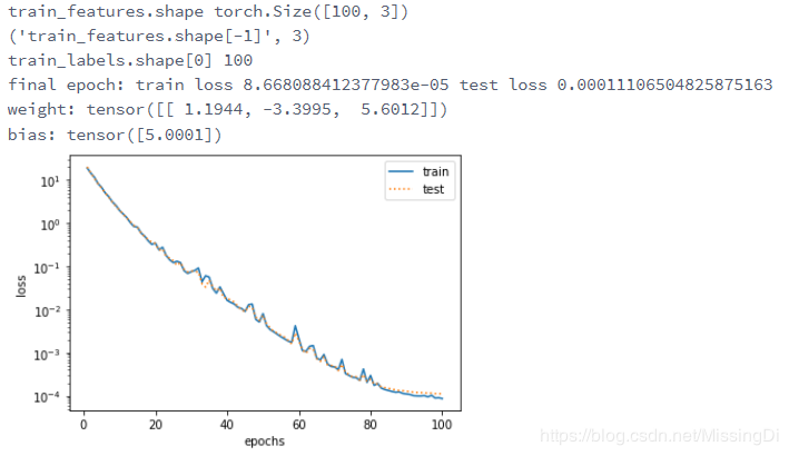
print('final epoch: train loss', train_ls[-1], 'test loss', test_ls[-1])
semilogy(range(1, num_epochs + 1), train_ls, 'epochs', 'loss',
range(1, num_epochs + 1), test_ls, ['train', 'test'])
print('weight:', net.weight.data,
'\nbias:', net.bias.data)
三阶多项式函数拟合(正常)
fit_and_plot(poly_features[:n_train, :], poly_features[n_train:, :], labels[:n_train], labels[n_train:]) # poly_features维度为(200, 3)
fit_and_plot(features[:n_train, :], features[n_train:, :], labels[:n_train], labels[n_train:]) # features维度为(200, 1)
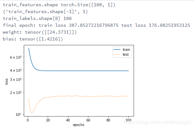
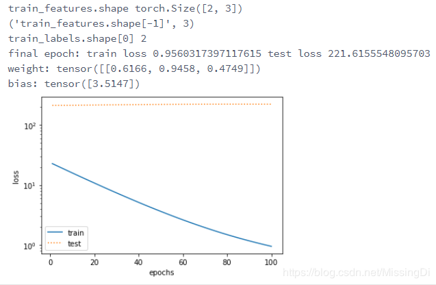
fit_and_plot(poly_features[0:2, :], poly_features[n_train:, :], labels[0:2], labels[n_train:])
权重衰减等价于 L2 范数正则化(regularization)。正则化通过为模型损失函数添加惩罚项使学出的模型参数值较小,是应对过拟合的常用手段。
L2 范数正则化(regularization)L2范数正则化在模型原损失函数基础上添加L2范数惩罚项,从而得到训练所需要最小化的函数。L2范数惩罚项指的是模型权重参数每个元素的平方和与一个正的常数的乘积。以线性回归中的线性回归损失函数为例:
其中w1,w2w_1,w_2w1,w2是权重参数,b是偏差参数,样本iii的输入为x1(i),x2(i)x_1^{(i)},x_2^{(i)}x1(i),x2(i),标签为y(i)y^{(i)}y(i),样本数为n。将权重参数用向量w=[w1,w2]w=[w_1,w_2]w=[w1,w2]表示,带有L2范数惩罚项的新损失函数为:
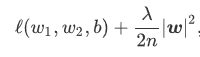
其中超参数λ>0。当权重参数均为0时,惩罚项最小。当λ较大时,惩罚项在损失函数中的比重较大,这通常会使学到的权重参数的元素较接近0。当λ设为0时,惩罚项完全不起作用。上式中L2范数平方∣w∣2|w|^2∣w∣2展开后得到w12+w22w_1^2+w_2^2w12+w22。
L2范数正则化又叫权重衰减。权重衰减通过惩罚绝对值较大的模型参数为需要学习的模型增加了限制,这可能对过拟合有效
详细例子见课程链接:
过拟合欠拟合及其解决方案
%matplotlib inline
import torch
import torch.nn as nn
import numpy as np
import sys
sys.path.append("/home/kesci/input")
import d2lzh1981 as d2l
print(torch.__version__)
def dropout(X, drop_prob):
    X = X.float()
    assert 0 <= drop_prob <= 1  #drop_prob的值必须在0-1之间,和数据库中的断言一个意思
    keep_prob = 1 - drop_prob
    # 这种情况下把全部元素都丢弃
    if keep_prob == 0:
        return torch.zeros_like(X)
    mask = (torch.rand(X.shape) < keep_prob).float()   # torch.rand()均匀分布,小于号<判别,若真,返回1,否则返回0
    # print('torch.rand(X.shape)',torch.rand(X.shape))
    return mask * X / keep_prob  # 重新计算新的隐藏单元的公式实现
X = torch.arange(16).view(2, 8)
# print(X)
dropout(X, 0)
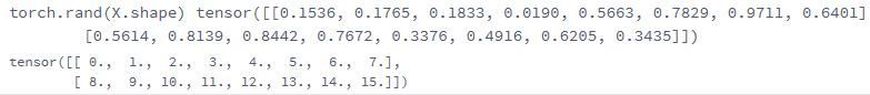
dropout(X, 0.5)
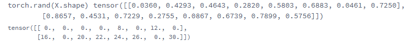
dropout(X, 1.0)
![]()
# 参数的初始化
num_inputs, num_outputs, num_hiddens1, num_hiddens2 = 784, 10, 256, 256
W1 = torch.tensor(np.random.normal(0, 0.01, size=(num_inputs, num_hiddens1)), dtype=torch.float, requires_grad=True)
b1 = torch.zeros(num_hiddens1, requires_grad=True)
W2 = torch.tensor(np.random.normal(0, 0.01, size=(num_hiddens1, num_hiddens2)), dtype=torch.float, requires_grad=True)
b2 = torch.zeros(num_hiddens2, requires_grad=True)
W3 = torch.tensor(np.random.normal(0, 0.01, size=(num_hiddens2, num_outputs)), dtype=torch.float, requires_grad=True)
b3 = torch.zeros(num_outputs, requires_grad=True)
params = [W1, b1, W2, b2, W3, b3]
drop_prob1, drop_prob2 = 0.2, 0.5
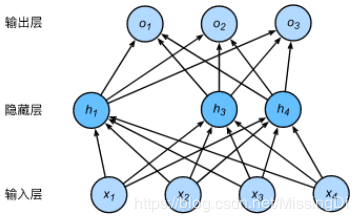
def net(X, is_training=True):
X = X.view(-1, num_inputs)
H1 = (torch.matmul(X, W1) + b1).relu()
if is_training: # 只在训练模型时使用丢弃法
H1 = dropout(H1, drop_prob1) # 在第一层全连接后添加丢弃层
H2 = (torch.matmul(H1, W2) + b2).relu()
if is_training:
H2 = dropout(H2, drop_prob2) # 在第二层全连接后添加丢弃层
return torch.matmul(H2, W3) + b3
def evaluate_accuracy(data_iter, net):
    acc_sum, n = 0.0, 0
    for X, y in data_iter:
        if isinstance(net, torch.nn.Module):  # instance(object,type)来判断一个对象(第一个参数(object))是否是一个已知的类型(第二个参数(type))
            net.eval() # 评估模式, 这会关闭dropout
            acc_sum += (net(X).argmax(dim=1) == y).float().sum().item()
            net.train() # 改回训练模式
        else: # 自定义的模型
            if('is_training' in net.__code__.co_varnames): # 如果有is_training这个参数
                # 将is_training设置成False
                acc_sum += (net(X, is_training=False).argmax(dim=1) == y).float().sum().item()
            else:
                acc_sum += (net(X).argmax(dim=1) == y).float().sum().item()
        n += y.shape[0]
    return acc_sum / n
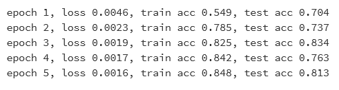
num_epochs, lr, batch_size = 5, 100.0, 256  # 这里的学习率设置的很大,原因与之前相同。
loss = torch.nn.CrossEntropyLoss()
train_iter, test_iter = d2l.load_data_fashion_mnist(batch_size, root='/home/kesci/input/FashionMNIST2065')
d2l.train_ch3(
    net,
    train_iter,
    test_iter,
    loss,
    num_epochs,
    batch_size,
    params,
    lr)
net = nn.Sequential(
        d2l.FlattenLayer(),
        nn.Linear(num_inputs, num_hiddens1),
        nn.ReLU(),
        nn.Dropout(drop_prob1),
        nn.Linear(num_hiddens1, num_hiddens2),
        nn.ReLU(),
        nn.Dropout(drop_prob2),
        nn.Linear(num_hiddens2, 10)
        )
for param in net.parameters():
    nn.init.normal_(param, mean=0, std=0.01)
optimizer = torch.optim.SGD(net.parameters(), lr=0.5)
d2l.train_ch3(net, train_iter, test_iter, loss, num_epochs, batch_size, None, None, optimizer)
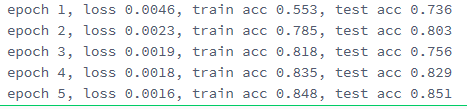
欠拟合现象:模型无法达到一个较低的误差
过拟合现象:训练误差较低但是泛化误差依然较高,二者相差较大
作者:MissingDi