RNN简单应用----预测正弦函数
利用RNN实现对函数sinx的取值预测,因为RNN模型预测的是离散时刻的取值,所以代码中需要将sin函数的曲线离散化,每隔一个时间段对sinx进行采样,采样得到的序列就是离散化的结果。
import numpy as np
import tensorflow as tf
import matplotlib.pyplot as plt
#定义参数
HIDDEN_SIZE = 30 # LSTM中隐藏节点的个数。
NUM_LAYERS = 2 # LSTM的层数。
TIMESTEPS = 10 # 循环神经网络的训练序列长度。
TRAINING_STEPS = 10000 # 训练轮数。
BATCH_SIZE = 32 # batch大小。
TRAINING_EXAMPLES = 10000 # 训练数据个数。
TESTING_EXAMPLES = 1000 # 测试数据个数。
SAMPLE_GAP = 0.01 # 采样间隔。
#产生正弦序列
def generate_data(seq):
X = []
y = []
# 序列的第i项和后面的TIMESTEPS-1项合在一起作为输入;第i + TIMESTEPS项作为输
# 出。即用sin函数前面的TIMESTEPS个点的信息,预测第i + TIMESTEPS个点的函数值。
for i in range(len(seq) - TIMESTEPS):
X.append([seq[i: i + TIMESTEPS]])
y.append([seq[i + TIMESTEPS]])
return np.array(X, dtype=np.float32), np.array(y, dtype=np.float32)
#定义模型结构
def lstm_model(X, y, is_training):
# 使用多层的LSTM结构。
cell = tf.nn.rnn_cell.MultiRNNCell([
tf.nn.rnn_cell.BasicLSTMCell(HIDDEN_SIZE)
for _ in range(NUM_LAYERS)])
# 使用TensorFlow接口将多层的LSTM结构连接成RNN网络并计算其前向传播结果。
outputs, _ = tf.nn.dynamic_rnn(cell, X, dtype=tf.float32)
output = outputs[:, -1, :]
# 对LSTM网络的输出再做加一层全链接层并计算损失。注意这里默认的损失为平均
# 平方差损失函数。
predictions = tf.contrib.layers.fully_connected(
output, 1, activation_fn=None)
# 只在训练时计算损失函数和优化步骤。测试时直接返回预测结果。
if not is_training:
return predictions, None, None
# 计算损失函数。
loss = tf.losses.mean_squared_error(labels=y, predictions=predictions)
# 创建模型优化器并得到优化步骤。
train_op = tf.contrib.layers.optimize_loss(
loss, tf.train.get_global_step(),
optimizer="Adagrad", learning_rate=0.1)
return predictions, loss, train_op
#定义训练函数
def train(sess, train_X, train_y):
ds = tf.data.Dataset.from_tensor_slices((train_X, train_y))
ds = ds.repeat().shuffle(1000).batch(BATCH_SIZE)
X, y = ds.make_one_shot_iterator().get_next()
# 调用模型,得到预测结果、损失函数和训练操作
with tf.variable_scope("model"):
predictions, loss, train_op = lstm_model(X, y, True)
# 初始化变量
sess.run(tf.global_variables_initializer())
for i in range(TRAINING_EXAMPLES):
_, l = sess.run([train_op, loss])
if i % 100 == 0:
print("train step:" + str(i) + ", loss: " + str(l))
def run_eval(sess, test_X, test_y):
# 将测试数据以数据集的方式提供给计算图。
ds = tf.data.Dataset.from_tensor_slices((test_X, test_y))
ds = ds.batch(1)
X, y = ds.make_one_shot_iterator().get_next()
# 调用模型得到计算结果。这里不需要输入真实的y值。
with tf.variable_scope("model", reuse=True):
prediction, _, _ = lstm_model(X, [0.0], False)
# 将预测结果存入一个数组。
predictions = []
labels = []
for i in range(TESTING_EXAMPLES):
p, l = sess.run([prediction, y])
predictions.append(p)
labels.append(l)
# 计算rmse作为评价指标。
predictions = np.array(predictions).squeeze()
labels = np.array(labels).squeeze()
rmse = np.sqrt(((predictions - labels) ** 2).mean(axis=0))
print("Root Mean Square Error is: %f" % rmse)
# 对预测的sin函数曲线进行绘图。
plt.figure()
plt.plot(predictions, label='predictions')
plt.plot(labels, label='real_sin')
plt.legend()
plt.show()
# 用正弦函数生成训练和测试数据集合。
test_start = (TRAINING_EXAMPLES + TIMESTEPS) * SAMPLE_GAP
test_end = test_start + (TESTING_EXAMPLES + TIMESTEPS) * SAMPLE_GAP
train_X, train_y = generate_data(np.sin(np.linspace(
0, test_start, TRAINING_EXAMPLES + TIMESTEPS, dtype=np.float32)))
test_X, test_y = generate_data(np.sin(np.linspace(
test_start, test_end, TESTING_EXAMPLES + TIMESTEPS, dtype=np.float32)))
with tf.Session() as sess:
# 训练模型
train(sess, train_X, train_y)
run_eval(sess, test_X, test_y)
训练输出: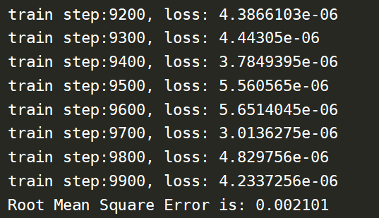
预测结果: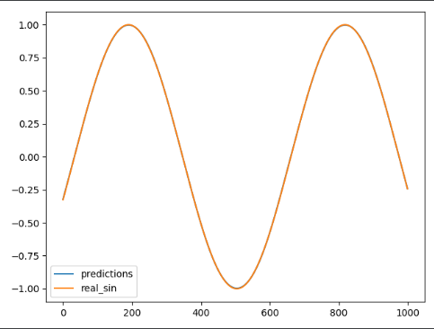
从曲线可以看出,预测得到的曲线和真实的sinx曲线完全重合,效果不错。
作者:Forizon
相关文章
Sally
2020-12-13
Tallulah
2023-07-20
Bea
2023-07-20
Ianthe
2023-07-20
Lani
2023-07-20
Thirza
2023-07-20
Rhoda
2023-07-20
Tesia
2023-07-20
Ursula
2023-07-20
Edana
2023-07-20
Dabria
2023-07-20
Paula
2023-07-20
Peony
2023-07-20
Rayna
2023-07-20
Fawn
2023-07-21
Tia
2023-07-21
Victoria
2023-07-21
Olathe
2023-07-21
Chipo
2023-07-21