数据挖掘TASK4_建模调参
建模与调参
作者:北海星
学习目标
掌握机器学习模型的建模与调参过程
内容介绍
线性回归模型:
线性回归对于特征的要求;
处理长尾分布;
理解线性回归模型;
模型性能验证:
评价函数与目标函数;
交叉验证方法;
留一验证方法;
针对时间序列问题的验证;
绘制学习率曲线;
绘制验证曲线;
嵌入式特征选择:
Lasso回归;
Ridge回归;
决策树;
模型对比:
常用线性模型;
常用非线性模型;
模型调参:
贪心调参方法;
网格调参方法;
贝叶斯调参方法;
代码示例
import pandas as pd
import numpy as np
import warnings
warnings.filterwarnings('ignore')
#定义reduce_men_usage函数,通过调整数据类型帮助我们减少数据所占内存空间
def reduce_mem_usage(df):
    start_men = df.memory_usage().sum()
    print('memory usage of dataframe is {:.2f} MB'.format(start_men))
    for col in df.columns:
        col_type = df[col].dtype
        if col_type != object:
            c_min = df[col].min()
            c_max = df[col].max()
            if str(col_type)[:3] == 'int':
                if c_min > np.iinfo(np.int8).min and c_max  np.iinfo(np.int16).min and c_max  np.iinfo(np.int32).min and c_max  np.iinfo(np.int64).min and c_max  np.finfo(np.float16).min and c_max  np.finfo(np.float32).min and c_max < np.finfo(np.float32).max:
                    df[col] = df[col].astype(np.float32)
                else:
                    df[col] = df[col].astype(np.float64)
        else:
            df[col] = df[col].astype('category')
    end_men = df.memory_usage().sum()
    print('Memory usage after optimization is :{:.2f} MB'.format(end_men))
    print('Decreased by {:.1f}%'.format(100*(start_men - end_men)/start_men))
    return df
sample_feature = reduce_mem_usage(pd.read_csv('data_for_tree.csv'))
#sample_feature.head()
memory usage of dataframe is 62099624.00 MB
Memory usage after optimization is :16520255.00 MB
Decreased by 73.4%
continuous_feature_names = [x for x in sample_feature.columns if x not in ['price','brand','model','brand']]
print(continuous_feature_names)
sample_feature = sample_feature.dropna().replace('-', 0).reset_index(drop=True)
sample_feature['notRepairedDamage'] = sample_feature['notRepairedDamage'].astype(np.float32)
train = sample_feature[continuous_feature_names + ['price']]
train_x = train[continuous_feature_names]
train_y = train['price']
['SaleID', 'name', 'bodyType', 'fuelType', 'gearbox', 'power', 'kilometer', 'notRepairedDamage', 'seller', 'offerType', 'v_0', 'v_1', 'v_2', 'v_3', 'v_4', 'v_5', 'v_6', 'v_7', 'v_8', 'v_9', 'v_10', 'v_11', 'v_12', 'v_13', 'v_14', 'train', 'used_time', 'city', 'brand_amount', 'brand_price_average', 'brand_price_max', 'brand_price_median', 'brand_price_min', 'brand_price_std', 'brand_price_sum', 'power_bin']
#train_x.head()
train_y.head()
0    1850.0
1    6222.0
2    5200.0
3    8000.0
4    3500.0
Name: price, dtype: float64
#1、简单建模,训练线性回归模型,查看截距与权重
from sklearn.linear_model import LinearRegression
model = LinearRegression(normalize=True)
model = model.fit(train_x, train_y)
sorted(dict(zip(continuous_feature_names, model.coef_)).items(), key=lambda x:x[1], reverse=True)
[('v_6', 3367064.341641952),
 ('v_8', 700675.5609398864),
 ('v_9', 170630.27723221222),
 ('v_7', 32322.661932025392),
 ('v_12', 20473.670796989394),
 ('v_3', 17868.07954151005),
 ('v_11', 11474.938996718518),
 ('v_13', 11261.764560017724),
 ('v_10', 2683.920090609242),
 ('gearbox', 881.8225039249613),
 ('fuelType', 363.90425072161565),
 ('bodyType', 189.60271012074494),
 ('city', 44.9497512052328),
 ('power', 28.55390161675131),
 ('brand_price_median', 0.5103728134078974),
 ('brand_price_std', 0.45036347092632434),
 ('brand_amount', 0.1488112039506708),
 ('brand_price_max', 0.0031910186703149753),
 ('SaleID', 5.3559899198567324e-05),
 ('seller', 2.4531036615371704e-06),
 ('train', 4.246830940246582e-07),
 ('offerType', -7.235445082187653e-06),
 ('brand_price_sum', -2.175006868187898e-05),
 ('name', -0.00029800127130847845),
 ('used_time', -0.0025158943328449923),
 ('brand_price_average', -0.40490484510113794),
 ('brand_price_min', -2.246775348688707),
 ('power_bin', -34.42064411726649),
 ('v_14', -274.7841180776088),
 ('kilometer', -372.897526660709),
 ('notRepairedDamage', -495.19038446298714),
 ('v_0', -2045.0549573540754),
 ('v_5', -11022.986240523212),
 ('v_4', -15121.731109858125),
 ('v_2', -26098.29992055678),
 ('v_1', -45556.189297264835)]
from matplotlib import pyplot as plt
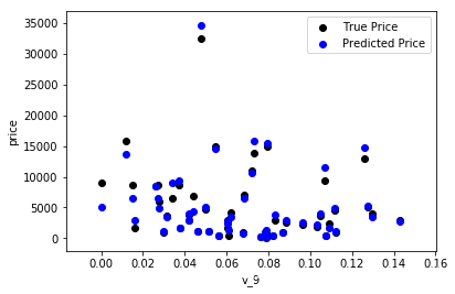
subsample_index = np.random.randint(low=0, high=len(train_y),size=50)#随机抽取50个点验证
plt.scatter(train_x['v_9'][subsample_index], train_y[subsample_index], color='black')
plt.scatter(train_x['v_9'][subsample_index], model.predict(train_x.loc[subsample_index]), color='blue')
plt.xlabel('v_9')
plt.ylabel('price')
plt.legend(['True Price','Predicted Price'],loc='upper right')
print('The predicted price is obvious different from true price')
plt.show()
The predicted price is obvious different from true price
import seaborn as sns
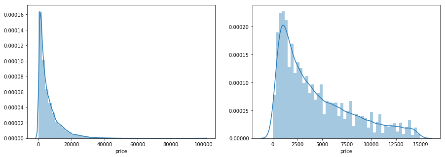
print('It is clear to see the price shows a typical exponential distribution')
plt.figure(figsize=(15,5))
plt.subplot(1,2,1)
sns.distplot(train_y)
plt.subplot(1,2,2)
sns.distplot(train_y[train_y < train_y.quantile(0.9)]) #将长尾截断
It is clear to see the price shows a typical exponential distribution
![[外链图片转存失败,源站可能有防盗链机制,建议将图片保存下来直接上传(img-qR3hcGGy-1585460408912)(output_7_3.png)]](/upload/wp-content/uploads/2020/03/20200329134844225.png)
#对标签进行log(x+1)变换使其贴近于正态分布,加一是为了防止底数为0
train_y_ln = np.log(train_y+1)
import seaborn as sns
print('The transformed price seems like normal distribution')
plt.figure(figsize=(15,5))
plt.subplot(1,2,1)
sns.distplot(train_y_ln)
plt.subplot(1,2,2)
sns.distplot(train_y_ln[train_y_ln < train_y.quantile(0.9)])
The transformed price seems like normal distribution
![[外链图片转存失败,源站可能有防盗链机制,建议将图片保存下来直接上传(img-4cBRUryw-1585460408915)(output_8_3.png)]](/upload/wp-content/uploads/2020/03/20200329134930218.png)
model = model.fit(train_x, train_y_ln)
print('intercept:'+str(model.intercept_))
sorted(dict(zip(continuous_feature_names, model.coef_)).items(), key=lambda x:x[1], reverse=True)
intercept:18.75074946557562
[('v_9', 8.052409900567515),
 ('v_5', 5.7642365966517515),
 ('v_12', 1.6182081236790782),
 ('v_1', 1.479831058296809),
 ('v_11', 1.1669016563609707),
 ('v_13', 0.9404711296034489),
 ('v_7', 0.713727308356328),
 ('v_3', 0.6837875771083226),
 ('v_0', 0.008500518010020237),
 ('power_bin', 0.00849796930289155),
 ('gearbox', 0.00792237727832305),
 ('fuelType', 0.006684769706828705),
 ('bodyType', 0.004523520092702963),
 ('power', 0.0007161894205359341),
 ('brand_price_min', 3.334351114747353e-05),
 ('brand_amount', 2.8978797042768103e-06),
 ('brand_price_median', 1.2571172872977267e-06),
 ('brand_price_std', 6.65917636342063e-07),
 ('brand_price_max', 6.194956307515807e-07),
 ('brand_price_average', 5.999345965093302e-07),
 ('SaleID', 2.1194170039646528e-08),
 ('seller', 9.978862181014847e-11),
 ('train', 7.958078640513122e-13),
 ('brand_price_sum', -1.5126504215909907e-10),
 ('offerType', -2.547437816247111e-10),
 ('name', -7.01551258888878e-08),
 ('used_time', -4.122479372354066e-06),
 ('city', -0.002218782481042724),
 ('v_14', -0.004234223418128389),
 ('kilometer', -0.013835866226882864),
 ('notRepairedDamage', -0.27027942349845646),
 ('v_4', -0.8315701200995309),
 ('v_2', -0.9470842241621843),
 ('v_10', -1.6261466689779176),
 ('v_8', -40.34300748761737),
 ('v_6', -238.79036385507334)]
plt.scatter(train_x['v_9'][subsample_index], train_y[subsample_index], color='black')
plt.scatter(train_x['v_9'][subsample_index], np.exp(model.predict(train_x.loc[subsample_index])), color='blue')
plt.xlabel('v_9')
plt.ylabel('price')
plt.legend(['True Price','Predicted Price'],loc='upper right')
print('The predicted price seems normal after np.log transforming')
plt.show()
The predicted price seems normal after np.log transforming
#2、五折交叉验证
#训练集,评估集,测试集。拿出训练集的一部分出来作为评估集,来对训练集生成的参数进行测试
from sklearn.model_selection import cross_val_score
from sklearn.metrics import mean_absolute_error,  make_scorer
def log_transfer(func):
    def wrapper(y, yhat):
        result = func(np.log(y),np.nan_to_num(np.log(yhat)))
        return result
    return wrapper
scores = cross_val_score(model, X=train_x, y=train_y, verbose=1, cv=5, scoring=make_scorer(log_transfer(mean_absolute_error)))
[Parallel(n_jobs=1)]: Done 5 out of 5 | elapsed: 0.7s finished
print('AVG:',np.mean(scores))
AVG: 1.3658023920313513
scores = pd.DataFrame(scores.reshape(1,-1))
scores.columns = ['cv' + str(x) for x in range(1, 6)]
scores.index = ['MAE']
scores
  cv1
  cv2
  cv3
  cv4
  cv5
  MAE
  1.348304
  1.36349
  1.380712
  1.378401
  1.358105
import numpy as np
np.reshape(scores, [1,-1])
scores.columns = ['cv' + str(x) for x in range(1, 6)]
scores.index = ['MAE']
scores
  cv1
  cv2
  cv3
  cv4
  cv5
  MAE
  1.348304
  1.36349
  1.380712
  1.378401
  1.358105
#3、模拟真实业务
#采用时间顺序对数据集进行分割,选靠前时间的4/5作为训练集,靠后的1/5作为验证集
sample_feature = sample_feature.reset_index(drop=True)
split_point = len(sample_feature)//5*4
train = sample_feature[:split_point].dropna()
val = sample_feature[split_point:].dropna()
train_x = train[continuous_feature_names]
train_y_ln = np.log(train['price'] + 1)
val_x = val[continuous_feature_names]
val_y_ln = np.log(val['price'] + 1)
model = model.fit(train_x, train_y_ln)
print('intercept:'+str(model.intercept_))
mean_absolute_error(val_y_ln, model.predict(val_x))
intercept:17.26478651939934
0.1957766416421094
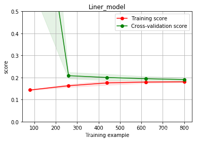
#4、绘制学习曲线
from sklearn.model_selection import learning_curve, validation_curve
def plot_learning_curve(estimator, title, X, y, ylim=None, cv=None,n_jobs=1, train_size=np.linspace(.1, 1.0, 5 )):
    plt.figure()
    plt.title(title)
    if ylim is not None:
        plt.ylim(*ylim)
    plt.xlabel('Training example')
    plt.ylabel('score')
    train_sizes, train_scores, test_scores = learning_curve(estimator, X, y, cv=cv, n_jobs=n_jobs, train_sizes=train_size, scoring = make_scorer(mean_absolute_error))
    train_scores_mean = np.mean(train_scores, axis=1)
    train_scores_std = np.std(train_scores, axis=1)
    test_scores_mean = np.mean(test_scores, axis=1)
    test_scores_std = np.std(test_scores, axis=1)
    plt.grid()#区域
    plt.fill_between(train_sizes, train_scores_mean - train_scores_std,
                     train_scores_mean + train_scores_std, alpha=0.1,
                     color="r")
    plt.fill_between(train_sizes, test_scores_mean - test_scores_std,
                     test_scores_mean + test_scores_std, alpha=0.1,
                     color="g")
    plt.plot(train_sizes, train_scores_mean, 'o-', color='r',
             label="Training score")
    plt.plot(train_sizes, test_scores_mean,'o-',color="g",
             label="Cross-validation score")
    plt.legend(loc="best")
    return plt
plot_learning_curve(LinearRegression(), 'Liner_model', train_x[:1000], train_y_ln[:1000], ylim=(0.0, 0.5), cv=5, n_jobs=1)
#模型调参
#1、通过线性回归,加入两种正则化方法,变成岭回归和Lasso回归
from sklearn.linear_model import LinearRegression
from sklearn.linear_model import Ridge
from sklearn.linear_model import Lasso
train = sample_feature[continuous_feature_names + ['price']].dropna()
train_X = train[continuous_feature_names]
train_y = train['price']
train_y_ln = np.log(train_y + 1)
#三种模型
result = {}
models = [LinearRegression(), Ridge(), Lasso()]
for model in models:
    model_name = str(model).split('(')[0]
    scores = cross_val_score(model, X=train_X, y=train_y_ln, verbose=0, cv=5, scoring=make_scorer(mean_absolute_error))
    result[model_name] = scores
    print(model_name+' is finished')
result = pd.DataFrame(result)
result.index = ['cv' + str(x) for x in range(1, 6)]
result
LinearRegression is finished
Ridge is finished
Lasso is finished
  LinearRegression
  Ridge
  Lasso
  cv1
  0.190792
  0.194832
  0.383899


  cv2
  0.193758
  0.197632
  0.381894


  cv3
  0.194132
  0.198123
  0.384090


  cv4
  0.191825
  0.195670
  0.380526


  cv5
  0.195758
  0.199676
  0.383611
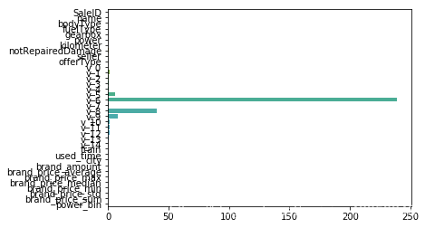
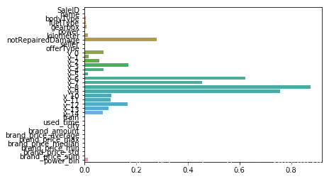
#线性回归
model = LinearRegression().fit(train_X, train_y_ln)
print('intercept:'+ str(model.intercept_))
sns.barplot(abs(model.coef_), continuous_feature_names)
intercept:18.750750028424832
#岭回归
model = Ridge().fit(train_X, train_y_ln)
print('intercept:'+ str(model.intercept_))
sns.barplot(abs(model.coef_), continuous_feature_names)
intercept:4.671709788130855
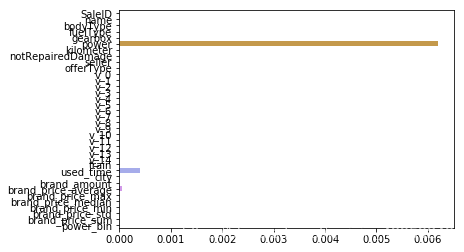
#LASSO回归
model = Lasso().fit(train_X, train_y_ln)
print('intercept:'+ str(model.intercept_))
sns.barplot(abs(model.coef_), continuous_feature_names)
intercept:8.67218477988307
#2、非线性回归
from sklearn.linear_model import LinearRegression
from sklearn.svm import SVC
from sklearn.tree import DecisionTreeRegressor
from sklearn.ensemble import RandomForestRegressor
from sklearn.ensemble import GradientBoostingRegressor
from sklearn.neural_network import MLPRegressor
from xgboost.sklearn import XGBRegressor
from lightgbm.sklearn import LGBMRegressor
models = [LinearRegression(),
          DecisionTreeRegressor(),
          RandomForestRegressor(),
          GradientBoostingRegressor(),
          MLPRegressor(solver='lbfgs', max_iter=100),
          XGBRegressor(n_estimators = 100, objective='reg:squarederror'),
          LGBMRegressor(n_estimators = 100)]
result = dict()
for model in models:
    model_name = str(model).split('(')[0]
    scores = cross_val_score(model, X=train_X, y=train_y_ln, verbose=0, cv = 5, scoring=make_scorer(mean_absolute_error))
    result[model_name] = scores
    print(model_name + ' is finished')
LinearRegression is finished
DecisionTreeRegressor is finished
RandomForestRegressor is finished
GradientBoostingRegressor is finished
MLPRegressor is finished
XGBRegressor is finished
LGBMRegressor is finished
result = pd.DataFrame(result)
result.index = ['cv' + str(x) for x in range(1, 6)]
result
  LinearRegression
  DecisionTreeRegressor
  RandomForestRegressor
  GradientBoostingRegressor
  MLPRegressor
  XGBRegressor
  LGBMRegressor
  cv1
  0.190792
  0.198679
  0.140822
  0.168900
  285.562549
  0.142367
  0.141542


  cv2
  0.193758
  0.193387
  0.143273
  0.171831
  572.989841
  0.140923
  0.145501


  cv3
  0.194132
  0.189258
  0.142621
  0.170875
  300.496953
  0.139393
  0.143887


  cv4
  0.191825
  0.190014
  0.142087
  0.169064
  2114.730472
  0.137492
  0.142497


  cv5
  0.195758
  0.204785
  0.144554
  0.174094
  353.180810
  0.143732
  0.144852
#模型调参
objective = ['regression', 'regression_l1', 'mape', 'huber', 'fair']
num_leaves = [3,5,10,15,20,40, 55]
max_depth = [3,5,10,15,20,40, 55]
bagging_fraction = []
feature_fraction = []
drop_rate = []
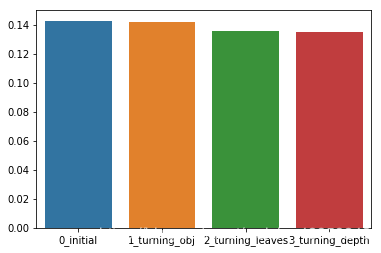
#1、贪心算法
best_obj = dict()
for obj in objective:
model = LGBMRegressor(objective=obj)
score = np.mean(cross_val_score(model, X=train_X, y=train_y_ln, verbose=0, cv = 5, scoring=make_scorer(mean_absolute_error)))
best_obj[obj] = score
best_leaves = dict()
for leaves in num_leaves:
model = LGBMRegressor(objective=min(best_obj.items(), key=lambda x:x[1])[0], num_leaves=leaves)
score = np.mean(cross_val_score(model, X=train_X, y=train_y_ln, verbose=0, cv = 5, scoring=make_scorer(mean_absolute_error)))
best_leaves[leaves] = score
best_depth = dict()
for depth in max_depth:
model = LGBMRegressor(objective=min(best_obj.items(), key=lambda x:x[1])[0],
num_leaves=min(best_leaves.items(), key=lambda x:x[1])[0],
max_depth=depth)
score = np.mean(cross_val_score(model, X=train_X, y=train_y_ln, verbose=0, cv = 5, scoring=make_scorer(mean_absolute_error)))
best_depth[depth] = score
sns.barplot(x=['0_initial','1_turning_obj','2_turning_leaves','3_turning_depth'], y=[0.143 ,min(best_obj.values()), min(best_leaves.values()), min(best_depth.values())])
#grid-search调参(穷举搜索)
from sklearn.model_selection import GridSearchCV
parameters = {'objective': objective , 'num_leaves': num_leaves, 'max_depth': max_depth}
model = LGBMRegressor()
clf = GridSearchCV(model, parameters, cv=5)
clf = clf.fit(train_X, train_y)
clf.best_params_
{'max_depth': 15, 'num_leaves': 55, 'objective': 'regression'}
model = LGBMRegressor(objective='regression',
                          num_leaves=55,
                          max_depth=15)
np.mean(cross_val_score(model, X=train_X, y=train_y_ln, verbose=0, cv = 5, scoring=make_scorer(mean_absolute_error)))
0.13754980533444577
#贝叶斯调参
from bayes_opt import BayesianOptimization
def rf_cv(num_leaves, max_depth, subsample, min_child_samples):
    val = cross_val_score(
        LGBMRegressor(objective = 'regression_l1',
            num_leaves=int(num_leaves),
            max_depth=int(max_depth),
            subsample = subsample,
            min_child_samples = int(min_child_samples)
        ),
        X=train_X, y=train_y_ln, verbose=0, cv = 5, scoring=make_scorer(mean_absolute_error)
    ).mean()
    return 1 - val
rf_bo = BayesianOptimization(
    rf_cv,
    {
    'num_leaves': (2, 100),
    'max_depth': (2, 100),
    'subsample': (0.1, 1),
    'min_child_samples' : (2, 100)
    }
)
rf_bo.maximize()
|   iter    |  target   | max_depth | min_ch... | num_le... | subsample |
-------------------------------------------------------------------------
| [0m 1       [0m | [0m 0.8625  [0m | [0m 98.27   [0m | [0m 16.21   [0m | [0m 46.74   [0m | [0m 0.5154  [0m |
| [95m 2       [0m | [95m 0.867   [0m | [95m 60.17   [0m | [95m 24.19   [0m | [95m 73.85   [0m | [95m 0.5303  [0m |
| [95m 3       [0m | [95m 0.8678  [0m | [95m 20.73   [0m | [95m 49.05   [0m | [95m 79.91   [0m | [95m 0.9991  [0m |
| [95m 4       [0m | [95m 0.8686  [0m | [95m 11.38   [0m | [95m 33.55   [0m | [95m 96.73   [0m | [95m 0.106   [0m |
| [0m 5       [0m | [0m 0.8583  [0m | [0m 28.24   [0m | [0m 88.14   [0m | [0m 32.07   [0m | [0m 0.54    [0m |
| [95m 6       [0m | [95m 0.8692  [0m | [95m 99.18   [0m | [95m 99.2    [0m | [95m 99.89   [0m | [95m 0.5816  [0m |
| [0m 7       [0m | [0m 0.8692  [0m | [0m 98.37   [0m | [0m 3.355   [0m | [0m 98.11   [0m | [0m 0.3583  [0m |
| [0m 8       [0m | [0m 0.8505  [0m | [0m 5.726   [0m | [0m 3.353   [0m | [0m 99.91   [0m | [0m 0.9506  [0m |
| [0m 9       [0m | [0m 0.8398  [0m | [0m 4.988   [0m | [0m 98.7    [0m | [0m 95.51   [0m | [0m 0.2637  [0m |
| [0m 10      [0m | [0m 0.802   [0m | [0m 98.82   [0m | [0m 96.37   [0m | [0m 3.977   [0m | [0m 0.7117  [0m |
| [0m 11      [0m | [0m 0.7719  [0m | [0m 6.261   [0m | [0m 12.23   [0m | [0m 2.926   [0m | [0m 0.9965  [0m |
| [0m 12      [0m | [0m 0.8668  [0m | [0m 56.81   [0m | [0m 23.78   [0m | [0m 71.71   [0m | [0m 0.1635  [0m |
| [0m 13      [0m | [0m 0.8684  [0m | [0m 99.3    [0m | [0m 46.5    [0m | [0m 86.75   [0m | [0m 0.1027  [0m |
| [95m 14      [0m | [95m 0.8693  [0m | [95m 51.32   [0m | [95m 77.08   [0m | [95m 99.54   [0m | [95m 0.1632  [0m |
| [0m 15      [0m | [0m 0.8678  [0m | [0m 17.64   [0m | [0m 47.26   [0m | [0m 78.37   [0m | [0m 0.5125  [0m |
| [0m 16      [0m | [0m 0.8654  [0m | [0m 67.56   [0m | [0m 99.3    [0m | [0m 62.61   [0m | [0m 0.1608  [0m |
| [95m 17      [0m | [95m 0.8694  [0m | [95m 48.5    [0m | [95m 43.38   [0m | [95m 99.52   [0m | [95m 0.1868  [0m |
| [0m 18      [0m | [0m 0.8632  [0m | [0m 57.29   [0m | [0m 61.38   [0m | [0m 49.45   [0m | [0m 0.2046  [0m |
| [0m 19      [0m | [0m 0.8666  [0m | [0m 95.77   [0m | [0m 3.698   [0m | [0m 71.83   [0m | [0m 0.5748  [0m |
| [0m 20      [0m | [0m 0.8689  [0m | [0m 85.61   [0m | [0m 76.58   [0m | [0m 98.76   [0m | [0m 0.6544  [0m |
| [0m 21      [0m | [0m 0.8692  [0m | [0m 70.03   [0m | [0m 98.23   [0m | [0m 99.73   [0m | [0m 0.3661  [0m |
| [0m 22      [0m | [0m 0.8692  [0m | [0m 97.84   [0m | [0m 27.73   [0m | [0m 99.84   [0m | [0m 0.212   [0m |
| [0m 23      [0m | [0m 0.8678  [0m | [0m 53.85   [0m | [0m 61.55   [0m | [0m 80.23   [0m | [0m 0.1136  [0m |
| [0m 24      [0m | [0m 0.8691  [0m | [0m 51.15   [0m | [0m 4.563   [0m | [0m 99.3    [0m | [0m 0.1271  [0m |
| [0m 25      [0m | [0m 0.8694  [0m | [0m 35.05   [0m | [0m 25.77   [0m | [0m 99.39   [0m | [0m 0.8209  [0m |
| [0m 26      [0m | [0m 0.8692  [0m | [0m 72.39   [0m | [0m 20.52   [0m | [0m 99.82   [0m | [0m 0.3174  [0m |
| [0m 27      [0m | [0m 0.8691  [0m | [0m 99.66   [0m | [0m 71.71   [0m | [0m 99.5    [0m | [0m 0.2219  [0m |
| [0m 28      [0m | [0m 0.8693  [0m | [0m 25.56   [0m | [0m 42.44   [0m | [0m 99.05   [0m | [0m 0.1066  [0m |
| [0m 29      [0m | [0m 0.8664  [0m | [0m 33.56   [0m | [0m 81.97   [0m | [0m 69.32   [0m | [0m 0.2377  [0m |
| [0m 30      [0m | [0m 0.868   [0m | [0m 87.97   [0m | [0m 93.77   [0m | [0m 85.64   [0m | [0m 0.1569  [0m |
=========================================================================
1 - rf_bo.max['target']
0.1305975267548991
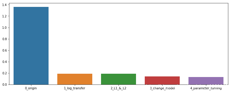
plt.figure(figsize=(13,5))
sns.barplot(x=['0_origin','1_log_transfer','2_L1_&_L2','3_change_model','4_parameter_turning'], y=[1.36 ,0.19, 0.19, 0.14, 0.13])
作者:北海星